Influence of Viscosity on Head Loss

Influence of Viscosity on Head Loss (US Customary Units)

Influence of Viscosity on Head Loss

Context: Fluid Flow in Pipes.

Transporting fluids (water, oil, gas, etc.) through pipelines is ubiquitous in industry and daily life. During this flow, the fluid rubs against the pipe walls, causing an energy loss known as head lossEnergy loss (often expressed in height of fluid column) experienced by a moving fluid, primarily due to friction.. This energy must be compensated for, often by a pump, which represents an energy cost. One of the fundamental fluid properties governing this energy loss is its viscosityA measure of a fluid's resistance to flow. A highly viscous fluid (like honey) flows with difficulty; a low-viscosity fluid (like water) flows easily.. This exercise aims to quantify and compare the head loss for two fluids with very different viscosities: water and oil.

Pedagogical Note: This exercise will teach you how to use the Reynolds number to characterize a flow and apply the Darcy-Weisbach formula to calculate an essential energy loss in the sizing of hydraulic systems.

Learning Objectives

Calculate the flow velocity and Reynolds number.
Determine the flow regime (laminar or turbulent).
Calculate the friction factor and the corresponding head loss.
Analyze and compare the impact of viscosity on the results.

Study Data

We want to compare the head loss generated by the flow of water and oil (SAE 30) in the same commercial steel pipe. The system is shown below.

Pipe System Diagram

Parameter	Symbol	Value	Unit
Pipe Length	\( L \)	328	ft
Internal Diameter	\( D \)	0.328	ft
Steel Roughness	\( \epsilon \)	0.00015	ft
Volumetric Flow Rate	\( Q \)	0.353	ft³/s
Acceleration of Gravity	\( g \)	32.2	ft/s²

Fluid Properties (at 20°C / 68°F)

Fluid	Density (\( \rho \))	Dynamic Viscosity (\( \mu \))
Water	1.94 slug/ft³	\( 2.09 \times 10^{-5} \) slug/(ft·s)
Oil SAE 30	1.77 slug/ft³	\( 0.00606 \) slug/(ft·s)

Problems to Solve

Calculate the average flow velocity \( V \) in the pipe.
For the water flow, calculate the Reynolds number \( Re_{\text{water}} \) and determine the nature of the flow regime (laminar or turbulent).
Using an appropriate formula, determine the friction factor \( f_{\text{water}} \).
Calculate the linear head loss \( h_{f,\text{water}} \) for the water.
Repeat steps 2 to 4 for the oil flow (\( Re_{\text{oil}}, f_{\text{oil}}, h_{f,\text{oil}} \)).
Compare the results and conclude on the influence of viscosity on head loss.

Fundamentals of Pipe Flow Hydraulics

To solve this exercise, several key concepts are necessary. They link the fluid properties, flow characteristics, and pipe geometry to quantify the energy lost.

1. Velocity and Flow Rate
The average velocity \(V\) of a fluid in a pipe with cross-sectional area \(A\) is related to the volumetric flow rate \(Q\) by the continuity equation. \[ V = \frac{Q}{A} \quad \text{with} \quad A = \frac{\pi D^2}{4} \]

2. Reynolds Number and Flow Regimes
The Reynolds number is a dimensionless quantity that characterizes the flow regime. It compares inertial forces to viscous forces. \[ Re = \frac{\rho V D}{\mu} \] Where \( \rho \) is the density, \( V \) is the velocity, \( D \) is the diameter, and \( \mu \) is the dynamic viscosity.

If \( Re < 2300 \), the flow is laminar.
If \( Re > 4000 \), the flow is turbulent.

3. Darcy-Weisbach Equation
This is the fundamental equation for calculating linear head loss (due to friction along the pipe's length). \[ h_f = f \frac{L}{D} \frac{V^2}{2g} \] Where \( f \) is the friction factor, which depends on the flow regime.

In laminar flow: \( f = \frac{64}{Re} \)
In turbulent flow, \( f \) depends on \( Re \) and the relative roughness \( \epsilon/D \). We use the Moody diagram or approximate formulas like the Swamee-Jain equation (very practical as it's explicit): \[ f = \frac{0.25}{\left[ \log_{10}\left( \frac{\epsilon/D}{3.7} + \frac{5.74}{Re^{0.9}} \right) \right]^2} \]

Solution: Influence of Viscosity on Head Loss

Question 1: Calculate the average flow velocity \( V \)

Principle (The Physics)

The velocity is the same for both fluids because they are transported at the same volumetric flow rate in the same pipe. This involves applying the continuity equation, which states that for an incompressible fluid, the flow rate is the product of velocity and cross-sectional area.

Mini-Lesson (Theoretical Deep Dive)

The conservation of mass, for a fluid of constant density \( \rho \) (incompressible), requires that the mass flow rate \( \dot{m} = \rho Q \) is constant. Consequently, the volumetric flow rate \( Q = A \times V \) is also constant. This is a fundamental principle in fluid mechanics.

Pedagogical Note (Instructor's Tip)

Always ensure your units are consistent before starting. Here, the flow rate is in m³/s and the diameter is in m, which is perfect. The most common error is forgetting to convert a diameter given in mm or cm.

Standards (The Engineering Reference)

Calculating velocity from flow rate is an application of basic physical principles (conservation of mass) and is not generally governed by a specific standard, but it is the first step in any standardized hydraulic calculation (e.g., ISO standards on flow measurement).

Formula(s) (The Mathematical Tool)

Velocity Formula

\begin{aligned} V &= \frac{Q}{A} \\ &= \frac{Q}{(\pi D^2 / 4)} \\ &= \frac{4Q}{\pi D^2} \end{aligned}

Assumptions (The Calculation Framework)

The flow is considered steady (flow rate does not change over time).
The calculated velocity is an average velocity over the cross-section; the actual velocity profile is not uniform.

Data (The Inputs)

Parameter	Symbol	Value	Unit
Volumetric Flow Rate	\(Q\)	0.353	ft³/s
Internal Diameter	\(D\)	0.328	ft

Tips (For Going Faster)

For a quick check, remember that \( \pi \approx 3.14 \). The calculation becomes \( (4 \times 0.353) / (3.14 \times 0.328^2) \approx 1.41 / (3.14 \times 0.107) \approx 1.41 / 0.336 \approx 4.2 \). This helps verify the order of magnitude of your result.

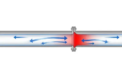
Diagram (Before Calculation)

The problem statement's diagram illustrates the situation well: a fluid with a known flow rate Q moving through a pipe of known diameter D.

Flow Representation

Calculation(s) (The Numerical Application)

Numerical Application of the Velocity Formula

First, let's calculate the cross-sectional area \(A\) of the pipe, which is the area of a circle with diameter \(D\).

\begin{aligned} A &= \frac{\pi D^2}{4} \\ A &= \frac{\pi \times (0.328 \text{ ft})^2}{4} \\ &= \frac{\pi \times 0.1076 \text{ ft²}}{4} \\ &\approx 0.0845 \text{ ft²} \end{aligned}

Now that we have the area \(A\), we can calculate the velocity \(V\) by dividing the volumetric flow rate \(Q\) by this area.

\begin{aligned} V &= \frac{Q}{A} \\ V &= \frac{0.353 \text{ ft³/s}}{0.0845 \text{ ft²}} \\ V &\approx 4.18 \text{ ft/s} \end{aligned}

Alternatively, using the direct formula (which combines the two previous steps), we can insert the values of \(Q\) and \(D\):

\begin{aligned} V &= \frac{4 \times Q}{\pi \times D^2} \\ V &= \frac{4 \times 0.353}{\pi \times (0.328)^2} \\ V &= \frac{1.412}{\pi \times 0.1076} \\ V &= \frac{1.412}{0.3379...} \\ V &\approx 4.18 \text{ ft/s} \end{aligned}

This confirms our previous result. The average fluid velocity in the pipe is 4.18 ft/s.

Diagram (After Calculation)

The actual velocity profile in the pipe depends on the flow regime, which will be determined in the next questions.

Possible Velocity Profiles

Analysis (Interpreting the Result)

A velocity of 4.18 ft/s is a common velocity for water flow in industrial pipes. This result is physically coherent.

Points of Caution (Mistakes to Avoid)

Be careful not to forget the square on the diameter in the area formula. This is a frequent error that skews all subsequent calculations.

Key Takeaways

The relationship \( Q = V \times A \) is fundamental.
The area of a circular pipe is \( A = \pi D^2 / 4 \).

Did You Know? (Engineering Culture)

The continuity principle is a form of the law of conservation of mass, one of the most fundamental principles in physics, formulated by Antoine Lavoisier in the 18th century: "Nothing is lost, nothing is created, everything is transformed."

FAQ (Clearing Up Doubts)

Final Result (The Bottom Line)

The average flow velocity in the pipe is 4.18 ft/s.

Your Turn (Check Your Understanding)

If the pipe diameter were doubled (D = 0.656 ft), what would the new velocity be for the same flow rate?

Question 2: Reynolds Number and Regime for Water

Principle (The Physics)

The Reynolds number determines whether inertial forces (which tend to create vortices) overcome viscous forces (which tend to dampen motion). Its value will place us in one of the flow regimes (laminar or turbulent).

Mini-Lesson (Theoretical Deep Dive)

The transition from laminar to turbulent flow is not instantaneous. There is a transition zone (generally between Re=2300 and Re=4000) where the flow is unstable and can oscillate between the two regimes. For engineering calculations, it is safely assumed that flow becomes turbulent as soon as Re > 2300.

Pedagogical Note (Instructor's Tip)

Remember the thresholds: 2300 for the end of laminar flow, 4000 for the beginning of fully turbulent flow. This is a universally accepted convention for circular pipes.

Standards (The Engineering Reference)

The definition of the Reynolds number and the transition thresholds are standardized and found in all technical literature and standards related to fluid mechanics (e.g., ISO 5167 on flow measurement).

Formula(s) (The Mathematical Tool)

Reynolds Number Formula

Re_{\text{water}} = \frac{\rho_{\text{water}} V D}{\mu_{\text{water}}}

Assumptions (The Calculation Framework)

Fluid properties (density, viscosity) are constant and correspond to a temperature of 20°C (68°F).
The pipe is assumed to be flowing full.

Data (The Inputs)

Parameter	Symbol	Value	Unit
Density (water)	\(\rho_{\text{water}}\)	1.94	slug/ft³
Velocity	\(V\)	4.18	ft/s
Diameter	\(D\)	0.328	ft
Dynamic Viscosity (water)	\(\mu_{\text{water}}\)	2.09 \times 10^{-5}	slug/(ft·s)

Tips (For Going Faster)

For water at room temperature, the kinematic viscosity is \( \nu = \mu / \rho \approx (2.09 \times 10^{-5}) / 1.94 \approx 1.08 \times 10^{-5} \) ft²/s. The formula becomes \( Re = VD/\nu \). This is often quicker.

Diagram (Before Calculation)

One can visualize turbulent flow as a collection of eddies and chaotic trajectories, unlike laminar flow where streamlines are parallel.

Visualization of Turbulent Regime

Calculation(s) (The Numerical Application)

Numerical Application for Water

We insert the values for water into the Reynolds formula. First, let's calculate the numerator (representing inertial forces).

\begin{aligned} \text{Numerator} &= \rho_{\text{water}} \times V \times D \\ \text{Numerator} &= 1.94 \text{ (slug/ft³)} \times 4.18 \text{ (ft/s)} \times 0.328 \text{ (ft)} \\ \text{Numerator} &\approx 2.661 \end{aligned}

Next, we divide this result by the dynamic viscosity \(\mu_{\text{water}}\) (representing viscous forces).

\begin{aligned} Re_{\text{water}} &= \frac{\text{Numerator}}{\mu_{\text{water}}} \\ Re_{\text{water}} &= \frac{2.661}{2.09 \times 10^{-5} \text{ (slug/(ft·s))}} \\ Re_{\text{water}} &\approx 127,320 \end{aligned}

The Reynolds number is therefore approximately 127,320. As this value is much greater than 4000, the regime is confirmed as turbulent.

Diagram (After Calculation)

The calculation confirms a turbulent regime. The associated velocity profile is "flatter" or "plug-like" in the center, compared to the parabolic profile of laminar flow.

Turbulent Velocity Profile

Analysis (Interpreting the Result)

The obtained value (127,320) is much higher than the 4000 threshold. The water flow is therefore clearly turbulent. Inertial forces are much more significant than viscous forces.

Points of Caution (Mistakes to Avoid)

Ensure you are using dynamic viscosity \( \mu \) (in slug/(ft·s)) and not kinematic viscosity \( \nu \) (in ft²/s) if the formula includes density \( \rho \). Do not mix the two formulas.

Key Takeaways

The Reynolds number is the key indicator of the flow regime.
\( Re < 2300 \Rightarrow \) Laminar, \( Re > 4000 \Rightarrow \) Turbulent.

Did You Know? (Engineering Culture)

The Reynolds number was introduced by George Stokes in 1851 but was popularized by Osborne Reynolds following his 1883 experiments that visualized the transition between laminar and turbulent regimes.

FAQ (Clearing Up Doubts)

Final Result (The Bottom Line)

The Reynolds number for water is approximately 127,320. The flow regime is turbulent.

Your Turn (Check Your Understanding)

If the water velocity were reduced to 0.0656 ft/s, what would the new Reynolds number be?

Question 3: Friction Factor for Water

Principle (The Physics)

The friction factor \(f\) is a dimensionless coefficient that quantifies the flow resistance due to wall roughness and turbulence. Since the flow is turbulent (as determined in Q2), this factor depends on both the Reynolds number and the pipe's relative roughness.

Mini-Lesson (Theoretical Deep Dive)

The Moody diagram is the most comprehensive graphical representation of the friction factor. It shows the three zones: laminar (a single line), critical (uncertainty zone), and turbulent. In the turbulent regime, we distinguish between "smooth" flow (where \(f\) depends only on Re) and "rough" flow (where \(f\) depends only on relative roughness for very high Re). Our case lies between these two.

Pedagogical Note (Instructor's Tip)

Learning to use an explicit formula like Swamee-Jain, or the implicit Colebrook equation, is essential for precise calculations, as reading from a Moody diagram can be imprecise. The Swamee-Jain formula is very convenient for spreadsheets or programs as it avoids iterative calculations.

Standards (The Engineering Reference)

Friction factor calculation formulas, like the Colebrook-White equation (from which Swamee-Jain is an approximation), are internationally recognized and form the basis for head loss calculations in many engineering codes and standards.

Formula(s) (The Mathematical Tool)

Swamee-Jain Equation (for turbulent flow)

f_{\text{water}} = \frac{0.25}{\left[ \log_{10}\left( \frac{\epsilon/D}{3.7} + \frac{5.74}{Re_{\text{water}}^{0.9}} \right) \right]^2}

Assumptions (The Calculation Framework)

The roughness of 0.00015 ft is an average value for new commercial steel. It can increase over time (corrosion, scaling).
The Swamee-Jain formula is a very accurate approximation of the Colebrook-White equation for \( 4000 < Re < 10^8 \).

Data (The Inputs)

Parameter	Symbol	Value	Unit
Roughness	\(\epsilon\)	0.00015	ft
Diameter	\(D\)	0.328	ft
Reynolds Number	\(Re_{\text{water}}\)	127320	-

Tips (For Going Faster)

For highly turbulent flows, the second term in the logarithm (\(5.74/Re^{0.9}\)) becomes negligible. You can quickly estimate \(f\) by considering only the roughness term, but the full calculation is preferable.

Diagram (Before Calculation)

This diagram shows how to find the friction factor on a Moody diagram. Start from the Reynolds number on the horizontal axis, move up to the curve corresponding to the relative roughness, then read the value of f on the vertical axis.

Reading the Moody Diagram (Principle)

Calculation(s) (The Numerical Application)

Calculation of Relative Roughness

The first step is to calculate the relative roughness, which is the dimensionless ratio of absolute roughness \(\epsilon\) to diameter \(D\).

\begin{aligned} \frac{\epsilon}{D} &= \frac{0.00015 \text{ ft}}{0.328 \text{ ft}} \\ &= 0.000457 \end{aligned}

Calculation of Friction Factor

We break down the calculation into several terms for clarity, using the Swamee-Jain formula:

f_{\text{water}} = \frac{0.25}{\left[ \log_{10}\left( \text{Term 1} + \text{Term 2} \right) \right]^2}

Term 1 (Roughness Influence): This term quantifies the effect of the wall's imperfections.

\begin{aligned} \text{Term 1} &= \frac{\epsilon/D}{3.7} \\ &= \frac{0.000457}{3.7} \\ &\approx 0.0001235 \end{aligned}

Term 2 (Reynolds Influence): This term quantifies the effect of turbulence. First, we calculate the denominator of this term:

\begin{aligned} \text{Denominator} &= Re_{\text{water}}^{0.9} \\ &= (127320)^{0.9} \\ &\approx 42090 \end{aligned}

Now we can calculate the full 'Term 2':

\begin{aligned} \text{Term 2} &= \frac{5.74}{\text{Denominator}} \\ &= \frac{5.74}{42090} \\ &\approx 0.0001364 \end{aligned}

Final Calculation: We add the two terms, take the base-10 logarithm, square the result, and divide 0.25 by that value.

\begin{aligned} f_{\text{water}} &= \frac{0.25}{\left[ \log_{10}\left( 0.0001235 + 0.0001364 \right) \right]^2} \\ &= \frac{0.25}{[ \log_{10}(0.0002599) ]^2} \\ &= \frac{0.25}{(-3.585)^2} \\ &= \frac{0.25}{12.85} \\ &\approx 0.01945 \end{aligned}

The friction factor for water is therefore approximately 0.0195.

Diagram (After Calculation)

The calculated point is located correctly in the turbulent zone of the Moody diagram, on the corresponding roughness curve.

Result Plot

Analysis (Interpreting the Result)

A friction factor of 0.0195 is a typical value for steel pipes with turbulent flow. The result is consistent.

Points of Caution (Mistakes to Avoid)

This formula uses the base-10 logarithm (\(\log_{10}\)), not the natural logarithm (\(\ln\)). Be careful what function you use on your calculator.

Key Takeaways

In the turbulent regime, the friction factor \(f\) depends on both \(Re\) and the relative roughness \(\epsilon/D\).

Did You Know? (Engineering Culture)

The Colebrook-White equation, from which the Swamee-Jain formula is derived, is implicit, meaning \(f\) cannot be solved for directly. Before modern calculators, solving it required tedious iterative methods (trial and error)!

FAQ (Clearing Up Doubts)

Final Result (The Bottom Line)

The friction factor for water is approximately 0.0195.

Your Turn (Check Your Understanding)

If the pipe were perfectly smooth (\(\epsilon = 0\)), what would the friction factor \(f_{\text{water}}\) be?

Question 4: Head Loss for Water

Principle (The Physics)

The linear head loss represents the energy per unit weight dissipated by fluid friction against the pipe walls over a given length. It is measured in meters (or feet) of the flowing fluid column.

Mini-Lesson (Theoretical Deep Dive)

A fluid's energy is often expressed by the Bernoulli equation. The head loss \(h_f\) is the term added to the Bernoulli equation between two points to account for real energy losses due to friction, which the ideal Bernoulli equation ignores.

Pedagogical Note (Instructor's Tip)

Pay close attention to the velocity term \(V^2 / (2g)\), known as the "velocity head". It represents the kinetic energy of the fluid. The head loss is proportional to this energy.

Standards (The Engineering Reference)

The Darcy-Weisbach equation is the standard method recommended by most plumbing and mechanical engineering codes for calculating head loss in pipes.

Formula(s) (The Mathematical Tool)

Darcy-Weisbach Equation

h_{f,\text{water}} = f_{\text{water}} \frac{L}{D} \frac{V^2}{2g}

Assumptions (The Calculation Framework)

The pipe is horizontal, so there is no change in elevation to consider.
We are only calculating "linear" (or "major") losses, due to the straight length of the pipe. "Minor" losses (from bends, valves, etc.) are not included.

Data (The Inputs)

Parameter	Symbol	Value	Unit
Friction Factor	\(f_{\text{water}}\)	0.0195	-
Length	\(L\)	328	ft
Diameter	\(D\)	0.328	ft
Velocity	\(V\)	4.18	ft/s
Gravity	\(g\)	32.2	ft/s²

Tips (For Going Faster)

First, calculate the \(L/D\) term (here, 1000) and the \(V^2/(2g)\) term (here, 0.271). This simplifies the final calculation and shows the influence of each part.

Diagram (Before Calculation)

We can imagine two pressure gauges (piezometer tubes) placed at the beginning and end of the pipe. The liquid level in the second tube will be lower than in the first, with the height difference corresponding to \(h_f\).

Visualizing Head Loss

Calculation(s) (The Numerical Application)

Applying Darcy-Weisbach

We calculate the terms of the formula separately for clarity.

Term 1: Friction Factor (from Q3)

f_{\text{water}} = 0.0195

Term 2: Geometric Ratio

\frac{L}{D} = \frac{328 \text{ ft}}{0.328 \text{ ft}} = 1000

Term 3: Velocity Head (Kinetic Energy)

\begin{aligned} \text{Term 3} &= \frac{V^2}{2g} \\ &= \frac{(4.18 \text{ ft/s})^2}{2 \times 32.2 \text{ ft/s²}} \\ &= \frac{17.47}{64.4} \\ &\approx 0.271 \text{ ft} \end{aligned}

Final Head Loss Calculation: We multiply the three terms together.

\begin{aligned} h_{f,\text{water}} &= f_{\text{water}} \times \left( \frac{L}{D} \right) \times \left( \frac{V^2}{2g} \right) \\ h_{f,\text{water}} &= 0.0195 \times 1000 \times 0.271 \\ h_{f,\text{water}} &= 19.5 \times 0.271 \\ h_{f,\text{water}} &\approx 5.28 \text{ ft} \end{aligned}

The total head loss for water over the 328 ft pipe is therefore 5.28 feet.

Diagram (After Calculation)

The previous diagram can be updated with the calculated value.

Calculated Head Loss for Water

Analysis (Interpreting the Result)

A head loss of 5.28 ft means that the flow over 328 ft of pipe has consumed as much energy as if the fluid had to be lifted to a height of 5.28 ft. This is a non-negligible value that must be compensated for by a pump.

Points of Caution (Mistakes to Avoid)

Don't forget to square the velocity. This is a very common source of error. Head loss is highly sensitive to velocity (it varies with \(V^2\)).

Key Takeaways

Head loss is proportional to the friction factor, the pipe length, and the square of the velocity, and inversely proportional to the diameter.

Did You Know? (Engineering Culture)

The unit "meters of fluid column" (or "feet of head") is very convenient because it is independent of the fluid's density when comparing energy. A loss of 10 m of water corresponds to a pressure drop of \( \rho_{\text{water}} g h \approx 1 \) bar, while a loss of 10 m of mercury corresponds to a pressure drop 13.6 times higher!

FAQ (Clearing Up Doubts)

Final Result (The Bottom Line)

The head loss for water is 5.28 feet.

Your Turn (Check Your Understanding)

If the velocity were doubled, by what factor would the head loss be multiplied (approximately)?

Question 5: Calculations for Oil (Re, f, hf)

Principle (The Physics)

We repeat the same sequence of calculations, but with the properties of oil. Since the viscosity is much higher, we expect viscous forces to dominate, which should radically change the nature of the flow and the associated energy losses.

Mini-Lesson (Theoretical Deep Dive)

In the laminar regime, friction no longer depends on the wall roughness. Fluid layers slide over one another, and the layer in contact with the wall is stationary. The energy loss is solely due to the fluid's internal "friction" (its viscosity) and not to turbulence or pipe imperfections.

Pedagogical Note (Instructor's Tip)

This is an excellent example showing that you cannot apply the same formula in every situation. The first step is ALWAYS to calculate the Reynolds number to know which "world" you are in: laminar or turbulent.

Standards (The Engineering Reference)

The formula \(f = 64/Re\) for the laminar regime in a circular pipe is an analytical solution to the Navier-Stokes equations, fundamental in fluid mechanics, and is therefore an absolute reference.

Formula(s) (The Mathematical Tool)

Calculation Sequence for Oil

Re_{\text{oil}} = \frac{\rho_{\text{oil}} V D}{\mu_{\text{oil}}} \quad \xrightarrow{Re < 2300} \quad f_{\text{oil}} = \frac{64}{Re_{\text{oil}}} \quad \Rightarrow \quad h_{f, \text{oil}} = f_{\text{oil}} \frac{L}{D} \frac{V^2}{2g}

Assumptions (The Calculation Framework)

The previous assumptions remain valid.
The viscosity of 0.00606 slug/(ft·s) for SAE 30 oil is a typical value at 20°C (68°F). This viscosity decreases very sharply with temperature.

Data (The Inputs)

Parameter	Symbol	Value	Unit
Density (oil)	\(\rho_{\text{oil}}\)	1.77	slug/ft³
Dynamic Viscosity (oil)	\(\mu_{\text{oil}}\)	0.00606	slug/(ft·s)
Velocity	\(V\)	4.18	ft/s
Diameter	\(D\)	0.328	ft
Length	\(L\)	328	ft
Gravity	\(g\)	32.2	ft/s²

Tips (For Going Faster)

By substituting the formulas, it can be shown that in the laminar regime, head loss is directly proportional to velocity V and viscosity µ, and no longer to the square of the velocity as in turbulent flow.

Diagram (Before Calculation)

The diagram represents laminar flow, where streamlines are parallel and orderly. This is the expected regime for a highly viscous fluid like oil at this velocity.

Visualization of Laminar Regime

Calculation(s) (The Numerical Application)

Step 1: Reynolds Number for Oil

First, we calculate the numerator (inertial forces) with the oil's properties. The velocity \(V\) and diameter \(D\) are the same as for water.

\begin{aligned} \text{Numerator} &= \rho_{\text{oil}} \times V \times D \\ \text{Numerator} &= 1.77 \text{ (slug/ft³)} \times 4.18 \text{ (ft/s)} \times 0.328 \text{ (ft)} \\ \text{Numerator} &\approx 2.427 \end{aligned}

Then, we divide by the oil's viscosity, which is much higher (0.00606 vs. 2.09e-5 for water).

\begin{aligned} Re_{\text{oil}} &= \frac{\text{Numerator}}{\mu_{\text{oil}}} \\ Re_{\text{oil}} &= \frac{2.427}{0.00606 \text{ (slug/(ft·s))}} \\ Re_{\text{oil}} &\approx 400.5 \end{aligned}

The result is 400.5. Since this value is well below the 2300 threshold, the flow is unambiguously laminar.

Step 2: Friction Factor for Oil

For the laminar regime, the friction factor calculation is direct and depends only on the Reynolds number. The pipe's roughness has no influence.

\begin{aligned} f_{\text{oil}} &= \frac{64}{Re_{\text{oil}}} \\ &= \frac{64}{400.5} \\ &\approx 0.1598 \text{ (rounded to 0.16)} \end{aligned}

Note that this friction factor (0.16) is much higher than that of water (0.0195).

Step 3: Head Loss for Oil

We use the Darcy-Weisbach equation again. The \(L/D\) (1000) and \(V^2/2g\) (0.271 ft) terms are identical to the water calculation, as the geometry and velocity are the same. Only the friction factor changes.

\begin{aligned} h_{f, \text{oil}} &= f_{\text{oil}} \times \left( \frac{L}{D} \right) \times \left( \frac{V^2}{2g} \right) \\ h_{f, \text{oil}} &= 0.1598 \times \left( \frac{328}{0.328} \right) \times (0.271) \\ h_{f, \text{oil}} &= 0.1598 \times 1000 \times 0.271 \\ h_{f, \text{oil}} &= 159.8 \times 0.271 \\ h_{f, \text{oil}} &\approx 43.3 \text{ ft} \end{aligned}

The head loss for the oil is therefore 43.3 feet, which is significantly higher than the 5.28 ft for water.

Diagram (After Calculation)

The laminar velocity profile is parabolic, with zero velocity at the wall and maximum velocity at the center. The head loss is also visualized.

Velocity Profile and Head Loss for Oil

Analysis (Interpreting the Result)

The friction factor for oil (0.16) is much higher than for water (0.0195). Consequently, the head loss is also much greater (43.3 ft vs. 5.28 ft). The high viscosity of the oil has "calmed" the flow (making it laminar) but has caused much stronger internal friction.

Points of Caution (Mistakes to Avoid)

The most serious error would be to apply the Swamee-Jain formula (for turbulent flow) to this laminar flow. The result would be completely wrong because it would account for pipe roughness, which has no influence here.

Key Takeaways

The methodology is crucial: 1. Velocity -> 2. Reynolds -> 3. Choose f formula -> 4. Calculate f -> 5. Calculate h_f.

Did You Know? (Engineering Culture)

Transporting highly viscous crude oil in pipelines often requires heating the fluid to lower its viscosity. Even though heating costs energy, it reduces head loss so much that the overall pumping cost is decreased!

FAQ (Clearing Up Doubts)

Final Result (The Bottom Line)

For the oil: \( Re \approx 401 \) (laminar), \( f \approx 0.16 \), and the head loss \( h_f \) is 43.3 feet.

Your Turn (Check Your Understanding)

If we used an oil twice as less viscous (\(\mu = 0.00303\) slug/(ft·s)), what would the new head loss be? (Be careful, the regime might change!)

Question 6: Comparison and Conclusion

Principle (The Physics)

This final step consists of synthesizing and interpreting the results obtained for both fluids to highlight the physical effect of viscosity on energy loss in an_flow.

Pedagogical Note (Instructor's Tip)

A comparison table is often the best tool to highlight differences and orders of magnitude. It allows for a quick visualization of a parameter's impact on the results.

Formula(s) (The Mathematical Tool)

No new formula; this is an analysis of the previous results.

Assumptions (The Calculation Framework)

The assumptions made previously condition this conclusion.

Data (The Inputs)

Parameter	Water	Oil
Reynolds Number	\(127,320\)	\(401\)
Friction Factor \(f\)	\(0.0195\)	\(0.16\)
Head Loss \(h_f\) (ft)	\(5.28\)	\(43.3\)

Diagram (Before Calculation)

This diagram places the two study cases side-by-side to prepare for the final comparison of their respective head losses.

Setup for Comparison

Diagram (After Calculation)

This bar chart visually compares the calculated head losses for water and oil, highlighting the enormous difference.

Head Loss Comparison

Analysis (Interpreting the Result)

Comparing the two situations, we observe major differences:

Parameter	Water	Oil	Ratio (Oil/Water)
Viscosity \( \mu \) (slug/(ft·s))	2.09 x 10⁻⁵	0.00606	~290x
Regime	Turbulent	Laminar	-
Friction Factor \( f \)	0.0195	0.16	~8.2x
Head Loss \( h_f \) (ft)	5.28	43.3	~8.2x

Despite having a slightly lower density, the oil, because its viscosity is 290 times higher than water's, generates more than 8 times the head loss. The flow regime is completely different, changing from turbulent to laminar, which radically alters how the friction factor is calculated. This demonstrates the critical influence of viscosity on the energy required to transport a fluid.

Key Takeaways

Conclusion on the Influence of Viscosity:

Viscosity is a dominant property in head loss calculation.
High viscosity tends to promote a laminar regime and significantly increases frictional forces.

Interactive Tool: Head Loss Simulator

Use the sliders to vary the fluid's viscosity and the flow rate. Observe the real-time impact on the Reynolds number, friction factor, and especially on the head loss. The graph shows the head loss evolution as a function of viscosity for the selected flow rate.

Input Parameters

Dynamic Viscosity (µ) in slug/(ft·s) (log scale) 2.09e-5 slug/(ft·s)

Flow Rate (Q) in ft³/s 0.35 ft³/s

Key Results (for L=328ft, D=0.328ft, ρ=1.94 slug/ft³)

Reynolds Number (Re) -

Flow Regime -

Friction Factor (f) -

Head Loss (h_f) in ft -

Glossary

Dynamic Viscosity (\( \mu \)): A fluid's property that measures its internal resistance to flow. The higher it is, the "thicker" the fluid and the more it resists motion. Unit: Pascal-second (Pa·s).
Head Loss (\( h_f \)): The loss of mechanical energy in a moving fluid, primarily due to friction against the pipe walls. It is expressed in units of length (e.g., meters or feet of fluid column).
Reynolds Number (Re): A dimensionless number that compares inertial forces to viscous forces. It is used to predict the flow regime of a fluid.
Laminar Regime: A flow regime at low velocity and/or high viscosity (Re < 2300), where fluid particles move in smooth, parallel, orderly layers.
Turbulent Regime: A flow regime at high velocity and/or low viscosity (Re > 4000), characterized by eddies and chaotic, disorderly motion of fluid particles.

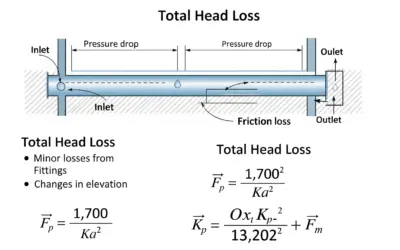
Total Head Loss in a Simple Pipe System

Fundamentals of Hydraulics

Exercise: Total Head Loss in a Simple Pipe System Calculating Total Head Loss in a Simple Pipe System Context: Water Flow in Pipes. In hydraulics, particularly in civil engineering fields like potable water supply or sanitation systems, it is crucial to understand and...

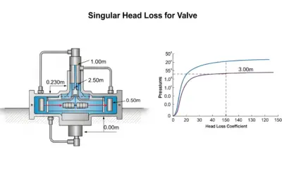
Calculating Singular Head Loss for a Valve

Fundamentals of Hydraulics

Exercise: Singular Head Loss for a Valve Calculating Singular Head Loss for a Valve Context: Singular Head LossLocalized energy losses in a hydraulic circuit, caused by pipe fittings (elbows, valves, tees, etc.) that disrupt the fluid flow.. In any hydraulic circuit,...

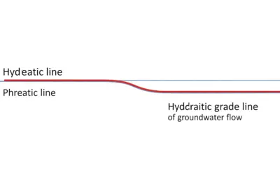
EGL and HGL Calculation

Fundamentals of Hydraulics

Exercise: EGL and HGL Calculation Calculating the Energy Grade Line (EGL) and Hydraulic Grade Line (HGL) Context: The study of pressurized pipe flowFlow of a fluid that completely fills a closed conduit. The pressure can be greater or less than atmospheric pressure.....

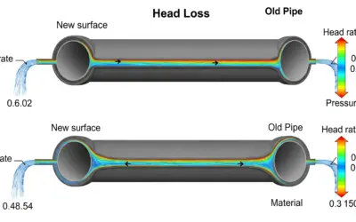
Comparison of Hydraulic Head Loss

Fundamentals of Hydraulics

Exercise: Comparing Hydraulic Head Loss Comparison of Hydraulic Head Loss Context: Fundamentals of Pressurized Pipe Flow. Transporting fluids in pipes is a pillar of civil and industrial engineering. However, as a fluid flows, it inevitably loses energy due to...

Calculating Power Dissipated by Head Loss

Fundamentals of Hydraulics

Exercise: Power Dissipated by Head Loss Calculating the Power Dissipated by Head Loss Context: Energy in Fluid Flow. When a fluid flows through a pipe, it loses energy due to friction against the walls (major head loss) and obstacles such as elbows, valves, or...

Head Loss Calculation with Hazen-Williams

Fundamentals of Hydraulics

Exercise: Head Loss Calculation with Hazen-Williams Head Loss Calculation with Hazen-Williams Context: Sizing a Water Supply Pipeline. One of the major challenges in hydraulic engineering is transporting water over long distances efficiently. To do this, it's crucial...

Falling Sphere Velocity according to Stokes’ Law

Fundamentals of Hydraulics

Exercise: Falling Sphere Velocity (Stokes' Law) Falling Sphere Velocity according to Stokes' Law Context: Studying Stokes' LawFormula expressing the drag force on a sphere moving in a viscous fluid at low velocity.. In fluid mechanics, understanding the motion of an...

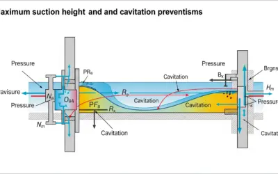
Calculating a Pump’s Maximum Suction Head

Fundamentals of Hydraulics

Calculating Maximum Suction Head Calculating a Pump's Maximum Suction Head Context: One of the biggest challenges in hydraulics is ensuring a pump operates correctly by avoiding the destructive phenomenon of cavitationThe formation of vapor bubbles in a liquid when...

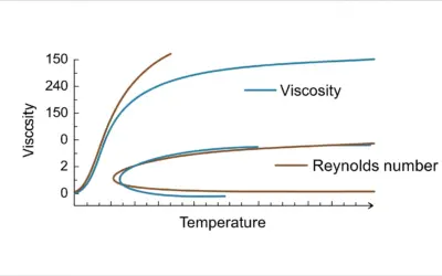
Analysis of Temperature Effects in Hydraulics

Fundamentals of Hydraulics

Exercise: Impact of Temperature on Head Loss Analysis of Temperature Effects in Hydraulics Context: The Impact of Thermal Variations on Hydraulic Systems. In many industrial applications, from petrochemicals to HVAC, fluids are transported at widely varying...

← Falling Sphere Velocity according to Stokes' Law Head Loss Calculation with Hazen-Williams →