Comparison of Hydraulic Head Loss
Context: Fundamentals of Pressurized Pipe Flow.
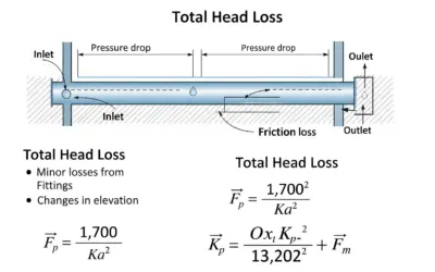
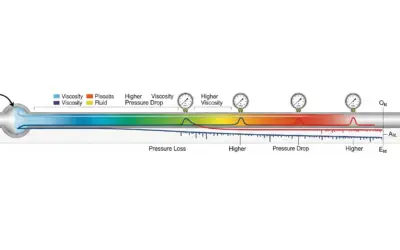
Transporting fluids in pipes is a pillar of civil and industrial engineering. However, as a fluid flows, it inevitably loses energy due to friction against the pipe walls (friction head lossDecrease in fluid pressure (head) during flow, due to friction on the pipe walls. Also known as linear or major loss.) and disturbances caused by pipe fittings like elbows, valves, or contractions (minor head lossEnergy loss due to flow disruption at a specific location, such as an elbow, valve, or tee. Also known as singular loss.). Calculating these losses accurately is crucial for correctly sizing pumps and ensuring the desired flow rate. This exercise aims to quantify and compare these two types of losses in simple network configurations.
Pedagogical Note: This exercise will teach you to break down a hydraulics problem, identify the different sources of energy loss, and apply the fundamental formulas to evaluate them. You will see the concrete impact that fittings can have on the total energy loss of a network.
Learning Objectives
- Differentiate and calculate friction (major) and minor head losses.
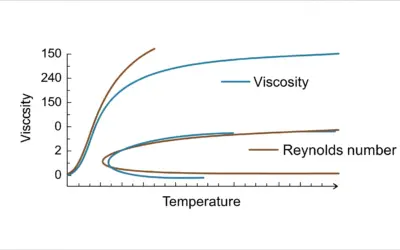
- Calculate the Reynolds numberA dimensionless quantity that characterizes the flow regime of a fluid (laminar, transitional, or turbulent). to determine the flow regime.
- Determine the Darcy friction factor using the Colebrook-White equation.
- Apply the Darcy-Weisbach equation to calculate friction head loss.
- Evaluate the impact of fittings (elbows, valves) on total head loss.
Problem Data
Configuration Diagram
| Characteristic | Symbol | Value | Unit |
|---|---|---|---|
| Fluid | - | Water | - |
| Water Temperature | \(T\) | 68 | °F |
| Kinematic Viscosity of Water | \(\nu\) | \(1.08 \times 10^{-5}\) | \(\text{ft}^2/\text{s}\) |
| Density of Water | \(\rho\) | 1.938 | \(\text{slug}/\text{ft}^3\) |
| Flow Rate | \(Q\) | 320 | \(\text{GPM}\) |
| Internal Pipe Diameter | \(D\) | 4.0 | \(\text{in}\) |
| Total Pipe Length | \(L\) | 160 | \(\text{ft}\) |
| Roughness of PVC | \(k\) | \(5 \times 10^{-6}\) | \(\text{ft}\) |
| Loss Coefficient (90° Elbow) | \(K_{\text{elbow}}\) | 0.9 | - |
| Loss Coefficient (Open Valve) | \(K_{\text{valve}}\) | 0.2 | - |
Questions
- Calculate the flow velocity and the Reynolds number. Is the flow laminar or turbulent?
- Determine the Darcy friction factor \(f\).
- Calculate the friction (major) head loss \(h_f\) for a length of 160 ft.
- Calculate the total minor head loss \(h_m\) for System B (which includes 2 elbows and 1 valve).
- Calculate the total head loss for each system and express the increase due to the fittings as a percentage.
Head Loss Fundamentals
1. Reynolds Number (\(Re\))
This dimensionless number compares inertial forces to viscous forces. It determines the flow regime:
- \(Re < 2000\): Laminar flow (ordered, smooth flow).
- \(Re > 4000\): Turbulent flow (chaotic flow, the most common case in engineering).
2. Friction (Major) Head Loss (\(h_f\))
This is the energy lost due to the fluid's friction along the length of the pipe. It is calculated with the Darcy-Weisbach equation:
\[ h_f = f \frac{L}{D} \frac{V^2}{2g} \]
Where \(f\) is the Darcy friction factor, \(L\) is length, \(D\) is diameter, \(V\) is velocity, and \(g\) is the acceleration of gravity (\(32.2 \text{ ft/s}^2\)).
3. Darcy Friction Factor (\(f\))
In turbulent flow, this coefficient depends on both the Reynolds number and the relative roughness (\(k/D\)). It is determined by the implicit Colebrook-White equation, which is often solved iteratively or using a Moody diagram.
\[ \frac{1}{\sqrt{f}} = -2 \log_{10}\left(\frac{k/D}{3.7} + \frac{2.51}{Re \sqrt{f}}\right) \]
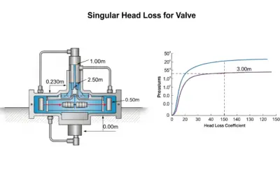
4. Minor Head Loss (\(h_m\))
This loss is generated by localized obstacles (fittings). Each fitting is characterized by a loss coefficient \(K\).
\[ h_m = K \frac{V^2}{2g} \]
The total minor loss is the sum of the losses from each fitting: \(h_{m, \text{total}} = \left(\sum K_i\right) \frac{V^2}{2g}\).
Solution: Comparison of Hydraulic Head Loss
Question 1: Flow Velocity and Reynolds Number
Principle
The first step is to determine the basic characteristics of the flow. Velocity is directly related to the flow rate and the pipe's cross-sectional area. The Reynolds number will then tell us the nature of the flow (laminar or turbulent), which is essential for choosing the correct method to calculate the friction factor.
Mini-Lesson
The continuity equation (\(Q=V \times A\)) expresses the conservation of mass for an incompressible fluid: flow rate is the product of velocity and area. The Reynolds number physically compares inertial forces (which tend to create chaos, i.e., turbulence) to viscous forces (which tend to dampen motion and keep it orderly).
Pedagogical Note
Always start a hydraulics problem with these two calculations. They set the stage. Knowing whether the flow is laminar or turbulent is like knowing the rules of a game before you start playing: it dictates all subsequent steps.
Standards
The Reynolds number transition thresholds (typically 2000 for the end of laminar flow and 4000 for the beginning of turbulent flow) are universally accepted conventions in fluid mechanics and are cited in nearly all technical manuals and standards in the field.
Formula(s)
Velocity Formula
Reynolds Number Formula
Assumptions
For these initial calculations, we make the following assumptions:
- The flow is incompressible (density \(\rho\) is constant).
- The flow is uniformly distributed across the pipe's cross-section (we use average velocity).
- The pipe is flowing full.
Given Data
| Parameter | Symbol | Value | Unit |
|---|---|---|---|
| Flow Rate | \(Q\) | 320 | \(\text{GPM}\) |
| Internal Diameter | \(D\) | 4.0 | \(\text{in}\) |
| Kinematic Viscosity | \(\nu\) | \(1.08 \times 10^{-5}\) | \(\text{ft}^2/\text{s}\) |
Tips
To quickly check your calculations, keep in mind that for common water distribution applications, pipe velocities are generally between 5 and 8 ft/s. Our result is in this range, which gives us confidence in the calculations.
Diagram (Before Calculations)
The following diagram illustrates the variables used to calculate velocity and Reynolds number in a pipe section.
Flow Parameters
Calculation(s)
Flow Rate Conversion
First, we convert all units to standard USCU for calculations: Gallons Per Minute (GPM) to cubic feet per second (ft³/s).
The flow rate to be used in the formulas is 0.713 ft³/s.
Diameter Conversion
We do the same for the diameter, converting it from inches (in) to feet (ft).
The diameter is 0.333 ft.
Cross-Sectional Area (A) Calculation
Now that we have the diameter in feet, we calculate the area of the circular pipe using the formula \(A = \pi D^2 / 4\).
The cross-sectional area for the flow is approximately 0.0871 ft².
Velocity (V) Calculation
The average velocity (V) is the flow rate (Q) divided by the area (A). We use the converted values.
The water velocity in the pipe is approximately 8.19 ft/s.
Reynolds Number (Re) Calculation
Finally, we calculate the Reynolds number (Re) to determine the flow regime, using velocity (V), diameter (D), and kinematic viscosity (\(\nu\)).
The result is \(Re \approx 252,500\). Since this number is much greater than 4000, the flow is definitively turbulent.
Diagram (After Calculations)
The calculation result places us in the turbulent flow regime, characterized by chaotic streamlines and eddies.
Flow Regime Visualization
Analysis
The Reynolds number is 252,500, which is much higher than 4000. The flow is therefore turbulent, as expected for a typical engineering application. We must use formulas suitable for turbulent flow for the rest of the problem.
Points of Caution
The most common error here is unit management. The flow rate is in GPM and the diameter in inches. It is imperative to convert everything to standard units (ft³/s and ft) before starting the calculations.
Key Takeaways
To master this step, remember:
- The fundamental relationship: Flow Rate = Velocity × Area (\(Q=V \cdot A\)).
- The Reynolds number formula: \(Re = VD/\nu\).
- The critical threshold: \(Re > 4000\) implies turbulent flow.
Did you know?
The experiment that visualized the transition between laminar and turbulent regimes was conducted in 1883 by British engineer Osborne Reynolds. He injected a fine stream of dye into water flowing through a glass tube, spectacularly showing the transition from a straight line (laminar) to chaotic eddies (turbulent).
FAQ
Final Answer
Try it yourself
Recalculate the velocity and Reynolds number if the flow rate were reduced to 80 GPM. Would the regime change?
Question 2: Darcy Friction Factor \(f\)
Principle
The Darcy friction factor \(f\) quantifies the intensity of energy loss due to friction. In turbulent flow, it depends on both the flow's turbulence (via the Reynolds number) and the pipe's surface condition (via the relative roughness).
Mini-Lesson
The Colebrook-White equation is the most accurate relationship for finding \(f\) in turbulent flow. Because it is implicit (\(f\) is on both sides), it cannot be solved directly. We use either numerical methods (iteration) or diagrams like the Moody diagram, which is a graphical representation of this equation.
Pedagogical Note
Don't be intimidated by the complexity of the Colebrook equation. Understand what it represents: a trade-off between the effect of viscosity (the Reynolds number term) and the effect of roughness (the k/D term). For very high Reynolds numbers, the flow is "fully turbulent," and \(f\) depends almost entirely on the roughness.
Standards
The Colebrook-White equation, although empirical, is the basis for most modern fluid dynamics calculations and is the foundation of the industry-standard Moody diagram.
Formula(s)
Colebrook-White Equation
Assumptions
We assume the provided roughness value \(k\) for PVC is accurate and constant over the entire pipe length. We also assume the pipe is new.
Given Data
| Parameter | Symbol | Value | Unit |
|---|---|---|---|
| PVC Roughness | \(k\) | 0.000005 | \(\text{ft}\) |
| Internal Diameter | \(D\) | 0.333 | \(\text{ft}\) |
| Reynolds Number | \(Re\) | 252,500 | - |
Tips
To avoid iteration, you can use explicit approximations like the Swamee-Jain equation, which is very accurate: \(f = 0.25 / [\log_{10}(k/(3.7D) + 5.74/Re^{0.9})]^2\). It gives a result almost identical to Colebrook for most applications.
Diagram (Before Calculations)
The following diagram represents the roughness \(k\) on the inner surface of the pipe with diameter \(D\).
Relative Roughness
Calculation(s)
Relative Roughness Calculation
The Colebrook equation uses relative roughness, which is the dimensionless ratio of roughness (k) to diameter (D).
This very low value confirms that the pipe is hydraulically smooth.
Solving Colebrook-White by Iteration
The Colebrook equation is implicit. We solve it by iteration. We start by guessing a value for \(f\), for example \(f_0 = 0.02\), and plug it into the right side of the equation to find a new value \(f_1\).
Iteration 1
Our first estimate \(f_1\) is 0.01467.
Iteration 2
We repeat the process: plug this new value \(f_1 = 0.01467\) into the right side of the equation to find \(f_2\).
We get \(f_2 \approx 0.01513\). The values are very close. We can stop iterating and use this value, which we'll round to \(f \approx 0.015\) for the subsequent calculations.
Diagram (After Calculations)
The Moody diagram helps visualize this result. We find our Reynolds number on the horizontal axis, move up to the curve matching our relative roughness, and then read the \(f\) value on the vertical axis.
Position on the Moody Diagram
Analysis
A friction factor \(f\) of 0.015 is typical for new PVC pipes under these flow conditions. It's a low value, confirming that PVC is a hydraulically "smooth" material. For rougher materials like concrete or corroded steel, \(f\) would be significantly higher.
Points of Caution
The main error is using roughness `k` in inches or mm instead of feet. All units in the Colebrook equation (except for the dimensionless Re) must be consistent (i.e., `k` and `D` must both be in feet).
Key Takeaways
- In turbulent flow, \(f\) depends on both Re and k/D.
- The Colebrook equation is the standard for calculating \(f\).
- The smoother the pipe (low k) and the more turbulent the flow (high Re), the lower \(f\) will be.
Did you know?
The Moody diagram, published in 1944 by Lewis Ferry Moody, was a revolution for engineers. It provided a graphical way to solve the complex Colebrook-White equation, which was essential before the age of calculators.
FAQ
Final Answer
Try it yourself
Calculate the new friction factor \(f\) if the pipe were new cast iron (\(k = 0.00085 \text{ ft}\)).
Question 3: Friction Head Loss \(h_f\)
Principle
Now that we have all the components (velocity, diameter, length, friction factor), we can directly apply the Darcy-Weisbach formula to quantify the energy lost solely due to friction over the 160-foot pipe length.
Mini-Lesson
The head loss \(h_f\) represents a loss of energy per unit weight of the fluid. This is why it has units of length (feet). It can be directly converted to pressure loss (\(\Delta P\)) using the relation \(\Delta P = \gamma h_f\), where \(\gamma\) is the specific weight of the fluid (\(62.4 \text{ lb/ft}^3\) for water).
Pedagogical Note
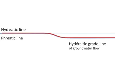
Think of friction head loss as an "energy slope." If you were to plot the energy grade line (EGL) along the pipe, it would slope downward at a constant, steady rate. This is the slope that pumps must overcome to maintain flow.
Standards
The Darcy-Weisbach equation is one of the most fundamental equations in hydraulics. It is universally recognized and forms the basis of all head loss calculations in engineering standards and design software.
Formula(s)
Darcy-Weisbach Equation
Assumptions
We assume that the flow conditions (velocity, diameter) and pipe properties (\(f\)) are constant over the entire length L.
Given Data
| Parameter | Symbol | Value | Unit |
|---|---|---|---|
| Friction factor | \(f\) | 0.015 | - |
| Length | \(L\) | 160 | \(\text{ft}\) |
| Diameter | \(D\) | 0.333 | \(\text{ft}\) |
| Velocity | \(V\) | 8.19 | \(\text{ft/s}\) |
| Gravity | \(g\) | 32.2 | \(\text{ft/s}^2\) |
Tips
The term \(V^2/(2g)\) is called the "velocity head." It represents the kinetic energy of the fluid. It's useful to calculate it once, as it is used for both friction and minor losses. This simplifies the calculations.
Diagram (Before Calculations)
The following diagram illustrates how the energy grade line (EGL) drops along a straight pipe due to friction head loss.
Illustration of Friction Head Loss
Calculation(s)
Velocity Head Calculation
The term \(V^2 / (2g)\) is the velocity head. We'll calculate it first since it's used for both major and minor losses.
The velocity head is approximately 1.041 ft.
Friction Head Loss Calculation
Now we apply the Darcy-Weisbach formula, plugging in all known values: \(f = 0.015\), \(L = 160 \text{ ft}\), \(D = 0.333 \text{ ft}\), and the velocity head \(V^2/(2g) \approx 1.041 \text{ ft}\).
The energy loss due to friction over the 160 ft pipe is 7.50 ft of head.
Diagram (After Calculations)
The EGL diagram is now updated with the calculated energy loss.
Friction Head Loss Value
Analysis
A loss of 7.50 feet means that to move the water over this 160-foot span, a pump would need to provide an additional pressure equivalent to a 7.50-foot column of water (about 3.25 psi), just to overcome friction.
Points of Caution
Ensure all units are consistent (feet, seconds). A common error is using the diameter in inches in the formula. Also, double-check that you are using the velocity V, not the flow rate Q, in the kinetic energy term.
Key Takeaways
- The Darcy-Weisbach equation is the central tool for friction losses.
- Friction losses are proportional to the length L and the square of the velocity V.
- The result \(h_f\) is a height (energy per unit weight), not a pressure.
Did you know?
Henry Darcy, a 19th-century French engineer, conducted experiments on water flowing through sand columns for the water supply of the city of Dijon. His work laid the foundation not only for head loss calculations in pipes but also for all of modern hydrogeology (Darcy's Law).
FAQ
Final Answer
Try it yourself
What would the friction head loss be if the pipe were 640 feet long instead of 160?
Question 4: Minor Head Loss \(h_m\) (System B)
Principle
System B contains fittings (elbows and a valve) that create local turbulence, generating additional energy losses. We must sum the dimensionless loss coefficients (K) for each fitting to get a total K-value, then use the minor loss formula which relates this loss to the fluid's kinetic energy.
Mini-Lesson
The loss coefficient K is an empirical value, determined in a lab. It represents the multiple of the velocity head (\(V^2/2g\)) that is "lost" as heat and turbulence when the fluid passes through the fitting. The more an accessory disturbs the flow (e.g., a half-closed valve), the higher its K value.
Pedagogical Note
Think of minor losses as "energy tolls." Every time the fluid encounters an obstacle, it has to "pay" a bit of its energy to pass. A straight pipe is a highway; a circuit with elbows and valves is a city road with traffic lights and intersections.
Standards
The K-values for standard fittings (elbows, tees, valves, etc.) are tabulated in numerous reference books and engineering standards, such as those from the Hydraulic Institute or in technical manuals like the Crane Technical Paper No. 410.
Formula(s)
Total Minor Head Loss
Assumptions
We assume the given K-values are correct and that the fittings are far enough apart that their turbulence effects do not interfere with each other.
Given Data
| Parameter | Symbol | Value | Unit |
|---|---|---|---|
| Coefficient (90° Elbow) | \(K_{\text{elbow}}\) | 0.9 | - |
| Coefficient (Open Valve) | \(K_{\text{valve}}\) | 0.2 | - |
| Velocity Head | \(V^2/2g\) | 1.041 | \(\text{ft}\) |
Tips
An alternative method for minor losses is the "equivalent length" (L_e) method. Each fitting is equated to a certain length of straight pipe that would produce the same loss (L_e = K * D / f). It's just another way of presenting the same calculation.
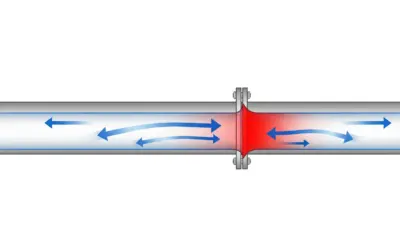
Diagram (Before Calculations)
Passing through an elbow forces the streamlines to bend, creating a separation zone and turbulence that dissipates energy.
Turbulence in an Elbow
Calculation(s)
Sum of K-Coefficients
To calculate the total minor loss, we first sum the K-values for all fittings in System B: two 90° elbows (\(K=0.9\)) and one open valve (\(K=0.2\)).
The total minor loss coefficient for this circuit is \(\sum K_i = 2.0\).
Minor Head Loss Calculation
We then use the minor loss formula, multiplying this total K-value by the velocity head (\(V^2/2g \approx 1.041 \text{ ft}\)) that we already calculated in Question 3.
The energy loss due to the three fittings is 2.08 ft of head.
Diagram (After Calculations)
The energy grade line experiences sharp drops at each fitting, corresponding to the localized energy loss.
Impact on the Energy Grade Line
Analysis
The loss from the fittings alone (2.08 ft) is a significant portion of the friction loss (7.50 ft). This illustrates that even in a relatively long pipe, ignoring minor losses can lead to a significant underestimation of the total losses.
Points of Caution
A common error is to forget a fitting in the sum of K-values, or to grab the wrong coefficient from reference tables (e.g., a 45° elbow instead of 90°).
Key Takeaways
- Minor losses are localized at fittings.
- They are calculated using a K-coefficient and the velocity head \(V^2/2g\).
- The total minor loss is the sum of the losses from each individual fitting.
Did you know?
A fully open butterfly valve or ball valve creates more head loss than a fully open gate valve of the same diameter, because their opening mechanism remains a larger obstruction in the flow path.
FAQ
Final Answer
Try it yourself
What would the minor head loss be if the valve were replaced with a globe valve (\(K=10\))?
Question 5: Comparison of Total Head Loss
Principle
The total head loss (`h_L`) of a network is simply the sum of the friction (major) losses (`h_f`) and the minor losses (`h_m`). By comparing the totals for both systems, we can quantify the real-world impact of adding a few elbows and a valve.
Mini-Lesson
The general energy equation (or extended Bernoulli's equation) states that the energy at point 1 equals the energy at point 2, plus any energy added by a pump (pump head), minus the energy lost (total head loss, `h_L`). Calculating \(h_L\) is therefore essential for determining the required pump power for a system.
Pedagogical Note
This final calculation is the synthesis of the entire exercise. It shows that network design is a trade-off. System A is more energy-efficient, but System B might be necessary to bypass an obstacle. The engineer must then quantify the energy "cost" of this geometric constraint.
Standards
The principle of adding friction and minor losses is a standard approach in all hydraulic network design methodologies. Professional simulation software applies this same fundamental principle.
Formula(s)
Total Head Loss
Assumptions
We assume there is no elevation change between the inlet and outlet of the systems so that the comparison focuses solely on friction and minor losses.
Given Data
| Parameter | Symbol | Value | Unit |
|---|---|---|---|
| Calculated Friction Loss | \(h_f\) | 7.50 | \(\text{ft}\) |
| Minor Loss (System B) | \(h_{m, B}\) | 2.08 | \(\text{ft}\) |
Tips
To quickly estimate the relative importance of losses, you can compare the sum of K-values (\(\sum K\)) to the friction term (\(f L/D\)). If \(\sum K\) is in the same order of magnitude as \(f L/D\), minor losses are significant. If \(f L/D\) is much larger, they are likely negligible.
Diagram (Before Calculations)
The following diagram conceptualizes the addition of friction and minor losses to get the total loss.
Composition of Total Head Loss
Calculation(s)
Total Loss for System A
The total loss for System A (straight pipe) is the sum of its friction loss (calculated in Q3) and its minor loss (which is zero, as there are no fittings).
Total Loss for System B
The total loss for System B is the sum of its friction loss (which is identical to System A, as the length L=160ft is the same) and its minor loss (calculated in Q4).
Percentage Increase Calculation
Finally, we calculate the percentage increase by comparing the difference in loss between the two systems (\(9.58 - 7.50\)) to the loss of the baseline system (System A).
Adding two elbows and a valve increased the total energy loss by 27.7%.
Diagram (After Calculations)
The chart clearly shows that the total head loss for System B is greater than for System A, with the increase entirely due to the red "Minor Loss" bar.
Head Loss Comparison
Analysis
Adding just three fittings increased the total energy loss by over 27%. This shows that minor losses, while localized, should never be neglected in hydraulic network design. They can have a considerable energy impact, translating directly to higher pump energy consumption.
Points of Caution
Don't compare apples to oranges. Ensure that the total length and diameter are the same for both systems so that the only variable being tested is the presence of fittings.
Key Takeaways
- Total head loss is the sum of friction (major) and minor losses.
- Fittings can account for a very large portion of the total energy loss, especially in short, complex networks.
- Optimizing a pipe layout to minimize bends and fittings is an effective strategy for reducing energy consumption.
Did you know?
In HVAC (Heating, Ventilation, and Air Conditioning) systems in large buildings, the ductwork networks are so complex (elbows, tees, dampers, filters) that minor losses often account for more than 75% of the total system head loss.
FAQ
Final Answer
Try it yourself
If the pipe were only 32 ft long instead of 160 ft, what would the new percentage increase be from the fittings?
Interactive Tool: Head Loss Simulator
Use the sliders to vary the flow rate and pipe diameter (for System B) and observe the impact on velocity, flow regime, and head loss.
Input Parameters
Key Results (System B)
Final Quiz: Test Your Knowledge
1. If you double the flow rate in a pipe, what happens to the approximate friction head loss?
2. What is the main characteristic of a laminar flow regime?
3. In the Darcy-Weisbach equation, the friction factor \(f\) depends on:
4. What does a "minor" head loss refer to?
5. To reduce friction head loss in an existing system without changing the flow rate, the most effective solution is:
Glossary
- Head Loss
- Represents the energy dissipation (pressure loss) of a moving fluid in a pipe. It is expressed in Pascals (Pa) or, more commonly, in feet of fluid head.
- Reynolds Number (Re)
- A dimensionless quantity used in fluid mechanics to characterize a flow regime. It helps predict whether the flow will be laminar or turbulent.
- Roughness (k)
- A measure of the texture of a pipe's inner surface. High roughness increases friction and thus friction head loss.
- Friction Head Loss (Major Loss)
- Energy loss due to the fluid's friction against the pipe walls over its entire length. Also called major or linear loss.
- Minor Head Loss
- Localized energy loss caused by flow disturbance when passing through a fitting (elbow, valve, tee, expansion, etc.). Also called singular loss.


0 Comments