Calculating the Power Dissipated by Head Loss
Context: Energy in Fluid Flow.
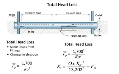
When a fluid flows through a pipe, it loses energy due to friction against the walls (major head loss) and obstacles such as elbows, valves, or expansions (minor head loss). This lost energy is converted into heat and must be compensated for, usually by a pump, to maintain the flow. Calculating the power dissipated by this head lossThe reduction in the total head (sum of elevation, pressure, and velocity head) of a fluid as it moves through a pipe system. is therefore a crucial step in designing hydraulic systems.
Pedagogical Note: This exercise will help you master the calculation of different head losses in a simple hydraulic circuit and quantify the energy needed to overcome them, a fundamental skill for any technician or engineer in fluid mechanics.
Learning Objectives
- Identify and differentiate between major (linear) and minor (singular) head losses.
- Calculate the flow velocity and the Reynolds number.
- Determine the friction factor using the Colebrook-White equation.
- Apply the Darcy-Weisbach formula for major losses.
- Calculate the sum of minor losses.
- Determine the hydraulic power (in horsepower) dissipated by the total head loss.
Problem Data
Hydraulic Circuit Diagram
| Parameter | Symbol | Value | Unit |
|---|---|---|---|
| Fluid | - | Water at 68°F | - |
| Water Specific Weight | \(\gamma\) | 62.4 | lb/ft³ |
| Water Kinematic Viscosity | \(\nu\) | \(1.06 \times 10^{-5}\) | ft²/s |
| Volume Flow Rate | \(Q\) | 220 | GPM |
| Inner Pipe Diameter | \(D\) | 3.94 | in |
| Total Pipe Length | \(L\) | 656.2 | ft |
| Absolute Pipe Roughness (PVC) | \(\varepsilon\) | \(5.0 \times 10^{-6}\) | ft |
| Loss Coefficient (90° Elbow) | \(K_{\text{elbow}}\) | 0.9 | - |
| Loss Coefficient (Valve) | \(K_{\text{valve}}\) | 0.2 | - |
| Acceleration of Gravity | \(g\) | 32.2 | ft/s² |
Questions to Solve
- Calculate the flow velocity \(V\) in the pipe.
- Calculate the Reynolds number \(Re\).
- Determine the friction factor \(f\).
- Calculate the major (linear) head loss \(\Delta H_{\text{lin}}\).
- Calculate the minor (singular) head loss \(\Delta H_{\text{sing}}\).
- Determine the total head loss \(\Delta H_{\text{tot}}\).
- Calculate the power \(P\) dissipated by the head loss (in horsepower).
Fundamentals of Head Loss
To solve this exercise, you must master the fundamental formulas for energy loss in pipes.
1. Major (Linear) Head Loss (Darcy-Weisbach)
This is caused by fluid friction along the length of the pipe. The Darcy-Weisbach equation is used to calculate it:
\[ \Delta H_{\text{lin}} = f \cdot \frac{L}{D} \cdot \frac{V^2}{2g} \]
Where \(f\) is the friction factor, \(L\) is the length, \(D\) is the diameter, \(V\) is the velocity, and \(g\) is the acceleration of gravity.
2. Minor (Singular) Head Loss
These are localized losses caused by pipe fittings (elbows, valves, etc.). They are calculated by summing the effects of each fitting:
\[ \Delta H_{\text{sing}} = \left( \sum K_i \right) \cdot \frac{V^2}{2g} \]
Where \(K_i\) is the loss coefficient for each component.
3. Dissipated Power (Water Horsepower)
The power lost (dissipated) to friction corresponds to the energy a pump must supply to overcome these losses. In USCS, this is often calculated in horsepower (hp).
\[ P \text{ (hp)} = \frac{\gamma \cdot Q \cdot \Delta H_{\text{tot}}}{550} \]
Where \(\gamma\) is the specific weight (lb/ft³), \(Q\) is the flow rate in **ft³/s**, \(\Delta H_{\text{tot}}\) is the total head loss in feet, and 550 is the conversion factor (550 ft·lb/s = 1 hp).
Solution: Calculating Power Dissipated by Head Loss
Question 1: Calculate the flow velocity \(V\)
Principle
The fluid velocity is the ratio of the volume flow rate (the volume of fluid passing through a cross-section per unit of time) to the area of that cross-section. It reflects how fast the fluid is moving.
Mini-Lesson
This calculation stems from the principle of conservation of mass for an incompressible fluid. The mass flow rate (\(\dot{m} = \rho \cdot Q\)) is constant. Since \(\rho\) is constant, the volume flow rate \(Q = A \cdot V\) is also constant. Velocity is therefore inversely proportional to the cross-sectional area.
Pedagogical Note
The first step in any USCS hydraulics calculation is to ensure all units are consistent. We must convert Gallons per Minute (GPM) to ft³/s and inches to feet before applying the formulas.
Standards
Common conversions in USCS are: 1 ft³ ≈ 7.48 gallons, and 1 ft = 12 inches. These are essential for all calculations.
Formula(s)
Velocity Formula
Area of a circular cross-section
Assumptions
We assume the fluid completely fills the pipe and the velocity is uniform across the cross-section (average velocity). In reality, the velocity is zero at the wall and maximum at the center (velocity profile).
Given Data
| Parameter | Symbol | Value | Unit |
|---|---|---|---|
| Volume Flow Rate | Q | 220 | GPM |
| Diameter | D | 3.94 | in |
Tips
For standard domestic or industrial water systems, flow velocity is often between 3 and 10 ft/s. A result far outside this range should alert you to a possible calculation error.
Diagram (Before Calculation)
Pipe Cross-Section and Flow Rate
Calculation(s)
1. Unit Conversion (to ft and s)
We convert the flow rate \(Q\) from GPM to ft³/s and the diameter \(D\) from inches to feet.
We now have our flow rate in ft³/s and our diameter in ft, ready for calculations.
2. Area Calculation (A)
We apply the area formula \(A = \frac{\pi D^2}{4}\) with the diameter in feet:
The cross-sectional area of our pipe is approximately 0.0845 square feet.
3. Velocity Calculation (V)
We apply the formula \(V = \frac{Q}{A}\) by substituting the converted values:
The final result for the average flow velocity is 5.80 ft/s.
Diagram (After Calculation)
Visualization of Velocity in the Pipe
Reflections
A velocity of 5.80 ft/s is a very plausible value for a pumping application, ensuring a good trade-off between reasonable head loss and an economical pipe diameter.
Caution
The most common error is mismatching units. Do not divide GPM by area in square inches! All units for primary equations (like \(V=Q/A\)) must be consistent (e.g., feet and seconds).
Key Takeaways
The fundamental relationship between flow rate, velocity, and area is key. Mastering unit conversions (GPM to ft³/s, inches to ft) is non-negotiable.
FAQ
Final Result
Your Turn
If the flow rate were 300 GPM with the same diameter, what would the new velocity be?
Hint: Velocity is directly proportional to the flow rate.
Question 2: Calculate the Reynolds number \(Re\)
Principle
The Reynolds number compares the magnitude of inertial forces (which tend to create turbulence) to that of viscous forces (which tend to dampen disturbances and maintain a smooth flow). It is the universal criterion for defining whether a flow is laminar or turbulent.
Mini-Lesson
A flow is said to be:
• Laminar (\(Re < 2000\)): Fluid particles slide past one another in orderly layers. Head loss is low.
• Transitional (\(2000 < Re < 4000\)): An unstable regime, difficult to predict.
• Turbulent (\(Re > 4000\)): The flow is chaotic, with eddies that significantly increase energy loss due to friction.
Pedagogical Note
Determining the flow regime is a mandatory step before you can choose the correct method for calculating the friction factor \(f\). Never skip this step!
Standards
The thresholds of 2000 and 4000 are empirically derived values universally recognized in fluid engineering codes and standards for internal flow in circular pipes.
Formula(s)
Reynolds Number Formula
Assumptions
We assume the fluid properties (\(\nu\)) are constant. In reality, viscosity depends on temperature, which can vary along the pipe.
Given Data
| Parameter | Symbol | Value | Unit |
|---|---|---|---|
| Velocity | V | 5.80 | ft/s |
| Diameter | D | 0.328 | ft |
| Kinematic Viscosity | \(\nu\) | 1.06 x 10⁻⁵ | ft²/s |
Tips
For water at room temperature in pipes a few inches in diameter, the flow becomes turbulent at very low velocities. In practice, most water applications are turbulent.
Diagram (Before Calculation)
Visualization of Flow Regimes
Calculation(s)
We apply the Reynolds number formula \( Re = \frac{V \cdot D}{\nu} \) using our consistent set of units (feet and seconds):
The Reynolds number is 179,500. Since this value is much greater than 4000, we confirm that the flow is turbulent.
Diagram (After Calculation)
Position on the Reynolds Scale
Reflections
With a value of 179,500, we are well within the turbulent regime. Inertial forces are 179,500 times more significant than viscous forces. Friction will therefore be significant and will depend on the pipe's roughness.
Caution
Ensure you are using kinematic viscosity (\(\nu\), in ft²/s). If you are given dynamic viscosity (\(\mu\), in lb·s/ft²), the formula changes to \(Re = \rho V D / \mu\), where \(\rho\) is the mass density (in slugs/ft³).
Key Takeaways
The Reynolds number is a prerequisite for calculating head loss. Remember the formula \(Re = VD/\nu\) and the regime change thresholds.
Did You Know?
Osborne Reynolds, an Irish engineer, first visualized the laminar-to-turbulent transition in 1883 by injecting a stream of dye into water flowing in a glass tube. His experiment is still replicated in engineering schools today.
FAQ
Final Result
Your Turn
If we were pumping an oil 5 times more viscous (\(\nu = 5.3 \times 10^{-5}\) ft²/s) at the same velocity, what would the new Reynolds number be?
Question 3: Determine the friction factor \(f\)
Principle
The friction factor \(f\) quantifies the intensity of head loss due to friction. In a turbulent regime, it depends on both the Reynolds number (which characterizes the flow) and the relative roughness of the pipe (which characterizes the wall).
Mini-Lesson
For turbulent flows, the relationship between \(f\), \(Re\), and the relative roughness \(\varepsilon/D\) is described by the Colebrook-White equation. This equation is implicit: the friction factor \(f\) appears on both sides, meaning it cannot be solved for directly. To solve it, we must use a numerical method, typically successive iterations.
Pedagogical Note
Choosing the roughness value \(\varepsilon\) is one of the biggest sources of uncertainty in hydraulic calculations. It depends on the material, its surface condition, and its age (corrosion, deposits). Always use reliable tabulated values.
Standards
Roughness values for various piping materials are provided by industrial standards (e.g., ASME, API) and manufacturers. The Darcy friction factor \(f\) used here is standard in US civil and mechanical engineering.
Formula(s)
Colebrook-White Equation
Assumptions
We assume the pipe roughness is uniform along its entire length.
Given Data
| Parameter | Symbol | Value | Unit |
|---|---|---|---|
| Absolute Roughness | \(\varepsilon\) | 5.0 x 10⁻⁶ | ft |
| Diameter | D | 0.328 | ft |
| Reynolds Number | Re | 179,500 | - |
Tips
To start the iterations, a good initial guess for \(f\) can be obtained from a simplified formula (like one for smooth pipes) or by using a typical value like 0.02.
Diagram (Before Calculation)
Principle of the Moody Diagram
Calculation(s)
1. Calculate Relative Roughness (\(\varepsilon/D\))
Both values are already in feet, so we can directly compute the dimensionless ratio.
This relative roughness of \(1.524 \times 10^{-5}\) is very low, confirming the pipe is "hydraulically smooth".
2. Iteration 1: Initial Guess
We start with an initial guess, \(f_0 = 0.02\). We plug this into the right-hand side of the Colebrook-White equation.
Our first guess \(f_0=0.02\) is refined to \(f_1 \approx 0.0157\). We use this new value for the next iteration.
3. Iteration 2: Refinement
We plug \(f_1 = 0.0157\) back into the equation.
The second iteration gives us \(f_2 \approx 0.0161\).
4. Iteration 3: Convergence
We repeat the process with \(f_2 = 0.0161\).
The third iteration gives \(f_3 \approx 0.0161\), which is the same as \(f_2\). The calculation has converged.
Diagram (After Calculation)
Reading from the Moody Diagram
Reflections
The value of 0.0161 is obtained by the reference method (Colebrook-White). Note that the original problem in SI units also yielded \(f=0.0161\). This shows that the friction factor is dimensionless, and as long as the inputs (\(Re\) and \(\varepsilon/D\)) are correct, the result is independent of the unit system.
Caution
Be careful to use the base-10 logarithm (\(\log_{10}\)) and not the natural logarithm (\(\ln\)). This is a common mistake when using calculators.
Key Takeaways
In a turbulent regime, the friction factor depends on \(Re\) and \(\varepsilon/D\). The Colebrook-White equation is the standard for calculating it and is solved by iteration.
Did You Know?
The Moody diagram, which is a graphical plot of the Colebrook-White equation, was the primary tool for solving this for decades before calculators and computers made iteration easy.
FAQ
Final Result
Your Turn
If the pipe were made of worn cast iron (\(\varepsilon = 0.00164\) ft), what would the new friction factor \(f\) be (keeping \(Re=179,500\))?
Question 4: Calculate the major (linear) head loss \(\Delta H_{\text{lin}}\)
Principle
Linear (or major) head loss represents the "continuous" energy loss due to the fluid's friction against the pipe walls along its entire length. It is often the most significant contribution to the total head loss in long pipelines.
Mini-Lesson
The Darcy-Weisbach formula shows that these losses increase with the square of the velocity. This means that doubling the flow rate (and thus the velocity) approximately quadruples the friction losses. They also increase linearly with length and inversely with diameter.
Pedagogical Note
The unit for \(\Delta H\) is feet. This should be interpreted as a "head" of fluid equivalent to the energy lost. If \(\Delta H = 10\) ft, it means the fluid lost as much energy as if it had fallen from a height of 10 feet.
Standards
The Darcy-Weisbach equation is the international standard for calculating linear head loss in pressurized pipes.
Formula(s)
Darcy-Weisbach Formula
Assumptions
We assume that the diameter, roughness, and flow rate are constant over the entire length \(L\).
Given Data
| Parameter | Symbol | Value | Unit |
|---|---|---|---|
| Friction Factor | f | 0.0161 | - |
| Length | L | 656.2 | ft |
| Diameter | D | 0.328 | ft |
| Velocity | V | 5.80 | ft/s |
| Gravity | g | 32.2 | ft/s² |
Tips
The term \(V^2 / (2g)\) is called the "velocity head". It is often useful to calculate it once and reuse it for both linear and singular loss calculations.
Diagram (Before Calculation)
Representation of a Straight Pipe
Calculation(s)
1. Calculate Velocity Head (a recurring term)
This term \( \frac{V^2}{2g} \) represents the fluid's kinetic energy per unit weight. It will be used again, so it's good to calculate it once:
This "velocity head" of 0.522 ft represents the fluid's velocity energy. We'll use this value in the next step.
2. Calculate Linear Head Loss
We apply the Darcy-Weisbach formula \( \Delta H_{\text{lin}} = f \cdot \frac{L}{D} \cdot \frac{V^2}{2g} \) by substituting all the values:
By multiplying the friction factor (f), the length-to-diameter ratio (L/D), and the velocity head, we get a total linear head loss of 16.81 feet.
Diagram (After Calculation)
Visualization of Linear Head Loss
Reflections
A loss of 16.81 feet means the pressure in the fluid has dropped by an amount equivalent to the pressure exerted by a 16.81 ft column of water (approx. 7.3 psi). This is a non-negligible energy loss.
Caution
Verify that all quantities in the Darcy-Weisbach formula are in consistent units (feet, ft/s, ft/s²) before doing the numerical application.
Key Takeaways
The Darcy-Weisbach equation is central to hydraulics. Remember the quadratic influence of velocity (\(V^2\)) and the influence of the \(L/D\) ratio.
Did You Know?
Henry Darcy was a 19th-century French engineer who conducted pioneering experiments on water flow through sand beds in Dijon, laying the foundations for modern hydrogeology and hydraulics.
FAQ
Final Result
Your Turn
If the pipe were 1312.4 ft long (double) instead of 656.2 ft, what would the new value of \(\Delta H_{\text{lin}}\) be?
Question 5: Calculate the minor (singular) head loss \(\Delta H_{\text{sing}}\)
Principle
Singular (or minor) head losses represent the "localized" energy loss caused by a disturbance in the flow. This disturbance is due to pipe fittings (elbows, valves, tees, reducers...) that force the fluid to change direction or velocity.
Mini-Lesson
Each fitting is characterized by a loss coefficient \(K\), which is a dimensionless number determined experimentally. The total head loss due to fittings is the sum of the individual losses, assuming the fittings are spaced far enough apart that their disturbances do not interfere with each other.
Pedagogical Note
In short circuits with many fittings (e.g., a mechanical room), minor losses can become dominant over major losses. Never neglect them without justification.
Standards
The \(K\) coefficients for standard fittings are tabulated in numerous fluid mechanics handbooks and professional standards (e.g., the Crane Technical Paper No. 410).
Formula(s)
Minor Head Loss Formula
Assumptions
We assume the K-factors provided by manufacturers are correct and that the fittings are far enough apart that their disturbance effects do not overlap in a complex way.
Given Data
| Parameter | Symbol | Value | Unit |
|---|---|---|---|
| Loss Coefficient (Elbow) | \(K_{\text{elbow}}\) | 0.9 | - |
| Loss Coefficient (Valve) | \(K_{\text{valve}}\) | 0.2 | - |
| Velocity Head | \(V^2/(2g)\) | 0.522 | ft |
Tips
A minor loss can also be expressed as an "equivalent length" of straight pipe: \(L_{\text{eq}} = K \cdot D/f\). This allows you to combine all losses into a single linear loss calculation over a total fictitious length.
Diagram (Before Calculation)
Location of Minor Losses
Calculation(s)
1. Sum of Loss Coefficients (K)
We add the K-factors for all fittings (2 elbows and 1 valve):
The sum of all K-factors for our fittings is 2.0 (dimensionless).
2. Calculate Minor Head Loss
We apply the formula \( \Delta H_{\text{sing}} = \left( \sum K_i \right) \cdot \frac{V^2}{2g} \). We reuse the velocity head \( \frac{V^2}{2g} \approx 0.522 \, \text{ft} \) calculated in step 4.
The energy loss due to fittings is 1.04 feet, which is small compared to the linear losses.
Diagram (After Calculation)
Drop in Energy Grade Line at Fittings
Reflections
The minor losses (1.04 ft) are much smaller than the major losses (16.81 ft) in this example because the pipe is long. This confirms that for long pipelines, linear friction losses are dominant.
Caution
Don't forget any fittings when counting the K-factors! A half-closed valve can have a K-factor of 5 or 10, radically changing the calculation.
Key Takeaways
The K-factor method is a simple and effective way to estimate localized losses. The loss is always proportional to the fluid's kinetic energy (\(V^2/2g\)).
Did You Know?
Golf balls have dimples for a reason related to head loss! These dimples create a thin turbulent boundary layer around the ball, which reduces "form drag" (a type of minor loss) and allows it to travel much farther than a smooth ball.
FAQ
Final Result
Your Turn
If we replaced the valve with a butterfly valve (K=1.5), what would the new \(\Delta H_{\text{sing}}\) be?
Question 6: Determine the total head loss \(\Delta H_{\text{tot}}\)
Principle
The total head loss is the sum of all energy losses experienced by the fluid along its path. It represents the total energy that the pump must supply to the fluid (per unit weight) just to maintain the flow, not counting any change in elevation or pressure between the inlet and outlet.
Mini-Lesson
In the generalized Bernoulli equation, which is the complete energy balance for a real fluid, \(\Delta H_{\text{tot}}\) appears as the loss term:
\(\frac{P_A}{\gamma} + \frac{V_A^2}{2g} + z_A + H_{\text{pump}} = \frac{P_B}{\gamma} + \frac{V_B^2}{2g} + z_B + \Delta H_{\text{tot}}\)
Pedagogical Note
This simple addition assumes that the disturbances from the fittings are spaced far enough apart not to interfere with each other. In practice, this is a very reliable approximation.
Formula(s)
Total Head Loss Formula
Assumptions
We assume that energy losses are additive, which is the standard assumption in hydraulics for pressurized flow.
Given Data
| Parameter | Symbol | Value | Unit |
|---|---|---|---|
| Major Head Loss | \(\Delta H_{\text{lin}}\) | 16.81 | ft |
| Minor Head Loss | \(\Delta H_{\text{sing}}\) | 1.04 | ft |
Diagram (Before Calculation)
Summing the Head Losses
Calculation(s)
We apply the formula \( \Delta H_{\text{tot}} = \Delta H_{\text{lin}} + \Delta H_{\text{sing}} \) by substituting the values from steps 4 and 5:
The total energy loss that the pump must overcome due to friction is 17.85 feet of water head.
Diagram (After Calculation)
Breakdown of Total Head Loss
Reflections
In this case (a long pipe), the major losses account for \(16.81 / 17.85 \approx 94\%\) of the total loss, while minor losses are only 6%. This justifies why minor losses can sometimes be neglected in very long pipelines, but major losses never can.
Caution
Ensure that \(\Delta H_{\text{lin}}\) and \(\Delta H_{\text{sing}}\) are in the same unit (feet) before adding them.
Key Takeaways
Total head loss is the sum of all major (friction over length) and minor (fittings) losses.
FAQ
Final Result
Your Turn
Using \(\Delta H_{\text{lin}} = 16.81\) ft and the answer from Your Turn #5 (with the butterfly valve, \(\Delta H_{\text{sing}}\) = 1.72 ft), what would the new \(\Delta H_{\text{tot}}\) be?
Question 7: Calculate the power \(P\) dissipated (in horsepower)
Principle
The dissipated power (or "water horsepower") is the amount of energy lost by the fluid to friction, per unit of time. This is the power that the pump must add to the fluid just to overcome the head loss.
Mini-Lesson
This power is converted into heat. The "brake horsepower" (BHP) of the pump, which is the actual power required from the motor, will be even higher, as you must account for the pump's efficiency (e.g., \(P_{\text{brake}} = P_{\text{water}} / \eta_{\text{pump}}\)).
Pedagogical Note
The conversion factor 1 hp = 550 ft·lb/s is a fundamental constant in USCS fluid dynamics and thermodynamics. Memorizing it is essential.
Standards
The standard unit for pump power in the US is horsepower (hp).
Formula(s)
Water Horsepower Formula
Assumptions
We assume the specific weight \(\gamma\) is constant throughout the circuit.
Given Data
| Parameter | Symbol | Value | Unit |
|---|---|---|---|
| Specific Weight | \(\gamma\) | 62.4 | lb/ft³ |
| Volume Flow Rate | Q | 0.490 | ft³/s |
| Total Head Loss | \(\Delta H_{\text{tot}}\) | 17.85 | ft |
| Conversion Factor | - | 550 | (ft·lb/s)/hp |
Tips
You will often see the formula with GPM: \(P \text{ (hp)} = \frac{\text{GPM} \cdot \Delta H_{\text{tot}} \cdot (\text{Sp. Gr.})}{3960}\). This is a derived formula that includes all the conversion factors (GPM to ft³/s, and \(\gamma\)). Let's check: \((220 \cdot 17.85 \cdot 1.0) / 3960 \approx 0.992 \text{ hp}\). It works! Our fundamental formula is more precise.
Diagram (Before Calculation)
Concept of Dissipated Power
Calculation(s)
First, we calculate the power in ft·lb/s using the formula \( P = \gamma \cdot Q \cdot \Delta H_{\text{tot}} \). We must use \(Q\) in ft³/s.
Next, we convert this value to horsepower by dividing by 550.
The product of these values gives us the dissipated power, which is approximately 0.993 horsepower.
Diagram (After Calculation)
Power Balance
Reflections
A power of 0.993 hp (or 741 W) is continuously converted into heat. The pump must supply at least this much "water horsepower". The actual "brake horsepower" required by the pump motor will be higher, e.g., if the pump is 75% efficient, the motor must provide \(0.993 / 0.75 \approx 1.32 \text{ hp}\).
Caution
The most common error is mismatching units in the power formula. Do NOT use GPM directly in the fundamental power equation. You must convert to ft³/s first, or use the "shortcut" formula (like the one in "Tips") which has the conversions built-in.
Key Takeaways
The water horsepower is the product of the fluid's specific weight (\(\gamma\)), the flow rate in ft³/s (\(Q\)), and the total head loss (\(\Delta H_{\text{tot}}\)), divided by 550.
Did You Know?
In large oil pipelines spanning thousands of miles, head losses are so significant that powerful pumping stations (often thousands of horsepower) must be installed every 50 to 100 miles to "re-boost" the pressure.
FAQ
Final Result
Your Turn
If the total head loss were 30 ft, what would the dissipated power be (in hp)?
Interactive Tool: Head Loss Simulator
Use the sliders to see how flow rate and pipe diameter influence the total head loss and dissipated power. Other parameters (length, roughness, etc.) remain fixed.
Input Parameters
Key Results
Final Quiz: Test Your Knowledge
1. What does the Reynolds number primarily represent?
2. Major (linear) head loss is directly proportional to:
3. What causes a minor (singular) head loss?
4. If you increase a pipe's roughness, the friction factor \(f\) for turbulent flow will:
5. In the US Customary System, a common unit for pump power is:
Glossary
- Head Loss
- Represents the energy loss (expressed as a height of fluid, in feet or meters) of a moving fluid due to friction.
- Reynolds Number (Re)
- A dimensionless number used in fluid mechanics to characterize a flow regime. It quantifies the ratio of inertial forces to viscous forces.
- Friction Factor (f)
- A dimensionless coefficient used in the calculation of linear head loss, which depends on pipe roughness and the Reynolds number.
- Roughness (\(\varepsilon\))
- A measure of the surface imperfections inside a pipe, which influences fluid friction.
- Specific Weight (\(\gamma\))
- The weight of a fluid per unit volume (e.g., lb/ft³). For water, this is approximately 62.4 lb/ft³.


0 Comments