Operating Point: Pumps in Series

Context: Pressurized Hydraulic SystemsSystems where fluid (like water) is conveyed under pressure, typically in closed pipes, requiring pumps to overcome elevation and friction..

In this exercise, we will analyze a common civil engineering problem: pumping water from a low-elevation source reservoir to a higher-elevation destination reservoir. The system requires a pump to overcome both the static elevation difference (static head) and the friction losses in the piping. We will determine the flow rate (the operating point) first for a single pump, and then analyze what happens when we install a second identical pump in series.

Pedagogical Note: This exercise will teach you how to graphically and algebraically combine pump performance curves with a system curve. This is a fundamental skill for designing water supply, irrigation, or industrial fluid transport systems, allowing engineers to correctly select pumps and predict system behavior.

Learning Objectives

Understand the concept of a hydraulic system curveA graphical representation of the total head required to move fluid through a piping system at various flow rates. It is the sum of static head and all friction losses. \(H_{\text{sys}} = H_{\text{static}} + H_{\text{friction}}\)..
Define a pump characteristic curveA graph provided by a pump manufacturer that shows the pump's performance, typically plotting head, efficiency, and NPSHr against a range of flow rates. using a simple equation.
Calculate the operating pointThe specific flow rate (Q) and head (H) where the pump's performance curve intersects the hydraulic system's resistance curve. This is the stable point at which the system will operate. for a single pump.
Determine the combined curve for two identical pumps in seriesA configuration where the discharge of one pump is connected to the suction of the next. This setup is used to add the head of each pump, achieving a higher total pressure..
Calculate the new operating point for the series configuration and compare the results.

Study Data

We need to pump water from a suction reservoir to a discharge reservoir. The system data and pump performance characteristics are as follows.

System Specifications

Characteristic	Value
Source Reservoir Water Level (WL)	100.0 ft
Destination Reservoir Water Level (WL)	120.0 ft
Piping System	Ductile Iron, 500 ft long, various fittings

System Overview

Parameter	Symbol	Value	Unit
Static Head (\(120 - 100\))	\(H_{\text{stat}}\)	20	ft
System Friction Coefficient	\(k\)	0.005	\(\text{ft/(GPM)}^2\)
Single Pump Shutoff Head	\(H_0\)	50	ft
Single Pump Curve Coefficient	\(c\)	0.01	\(\text{ft/(GPM)}^2\)

Questions to Address

Define the system curve equation \(H_{\text{sys}} = f(Q)\) and the single pump curve equation \(H_{\text{pump},1} = f(Q)\).
Calculate the operating point (Flow \(Q\) in GPM, Head \(H\) in ft) for a single pump.
Define the combined pump curve equation \(H_{\text{pump},2} = f(Q)\) for two identical pumps in series.
Calculate the new operating point (Flow \(Q\) in GPM, Head \(H\) in ft) for the two pumps in series.
Compare and analyze the results from Question 2 and Question 4.

Fundamentals of Hydraulic Systems

To solve this problem, we need to understand two key concepts: the System Curve and the Pump Curve.

1. The System Curve (\(H_{\text{sys}}\))
The system curve represents the total head (energy) a pump must generate to move fluid through a specific piping system. It is the sum of the static head (the physical elevation change) and the friction losses (head lost to friction in pipes and fittings). Friction losses are typically proportional to the square of the flow rate (\(Q\)). \[ H_{\text{sys}} = H_{\text{static}} + H_{\text{friction}} \] \[ H_{\text{sys}} = H_{\text{static}} + k \cdot Q^2 \]

2. Pumps in Series
When two or more pumps are placed in series (the discharge of one feeds the suction of the next), their individual heads are added together at any given flow rate. This configuration is used to overcome a higher total head than a single pump can achieve. \[ H_{\text{series}}(Q) = H_{\text{pumpA}}(Q) + H_{\text{pumpB}}(Q) \] For two identical pumps: \(H_{\text{series}}(Q) = 2 \cdot H_{\text{pump},1}(Q)\)

Solution: Operating Point: Pumps in Series

Question 1: Define System & Single Pump Curves

Principle

The first step is to mathematically describe both the system's resistance to flow (System Curve) and the pump's performance (Pump Curve) using the given formulas and data. This establishes the "demand" (system) and "supply" (pump) for our energy balance.

Mini-Lesson

Parabolic Models: Both pump curves and system curves are often simplified as parabolic (quadratic) equations of the form \(H = A \pm B \cdot Q^2\). This is a good approximation for turbulent flow (where friction is proportional to \(Q^2\)) and the typical performance of a centrifugal pump.

Pedagogical Note

Think of this step as defining the two "players" in this problem: the pipeline (system) and the machine (pump). We need to know the rules they play by (their equations) before we can see how they interact.

Norms

Pump performance curves are typically developed according to standards from the Hydraulic Institute (HI). System curve calculations are based on fundamental fluid mechanics principles (e.g., the Darcy-Weisbach equation).

Formula(s)

We will use the standard equations provided in the fundamentals section.

System Curve Formula

H_{\text{sys}} = H_{\text{static}} + k \cdot Q^2

Pump Curve Formula (simplified model)

H_{\text{pump},1} = H_0 - c \cdot Q^2

Hypotheses

We make the following assumptions for this calculation:

The flow is fully turbulent, so friction is proportional to \(Q^2\).
The fluid (water) has constant density and viscosity.
The reservoir levels are constant.
The provided parabolic equations are accurate models for the pump and system.

Data

From the problem statement:

Parameter	Symbol	Value	Unit
Static Head	\(H_{\text{stat}}\)	20	ft
Friction Coefficient	\(k\)	0.005	\(\text{ft/(GPM)}^2\)
Shutoff Head	\(H_0\)	50	ft
Pump Coefficient	\(c\)	0.01	\(\text{ft/(GPM)}^2\)

Tips

The units are critical. Notice that the coefficients \(k\) and \(c\) are given in "ft per GPM squared". This confirms they are meant to be multiplied by \(Q^2\) (in GPM²) to get a result in feet (ft), which correctly adds to the other head values.

Calculation(s)

We will substitute the known values from the 'Data' section into the general formulas.

Step 1: Define System Curve

We start with the general formula \(H_{\text{sys}} = H_{\text{static}} + k \cdot Q^2\) and substitute the given values: \(H_{\text{static}} = 20\) ft and \(k = 0.005\).

H_{\text{sys}} = 20 + 0.005 \cdot Q^2

This equation now represents the total head the system requires for any flow Q.

Step 2: Define Single Pump Curve

Similarly, we use the general pump formula \(H_{\text{pump},1} = H_0 - c \cdot Q^2\) and substitute the pump's specific values: \(H_0 = 50\) ft and \(c = 0.01\).

H_{\text{pump},1} = 50 - 0.01 \cdot Q^2

This equation represents the total head the single pump can supply at any flow Q.

Analysis

We now have two distinct equations. The \(H_{\text{sys}}\) equation tells us the head required (demand) for any flow \(Q\), and it *increases* with flow. The \(H_{\text{pump},1}\) equation tells us the head supplied (supply) for any flow \(Q\), and it *decreases* with flow.

Cautionary Points

Be careful not to mix up the system coefficient (\(k\)) and the pump coefficient (\(c\)). One describes the piping, the other describes the pump.

Key Takeaways

System Curve (Demand): \(H_{\text{sys}} = H_{\text{static}} + H_{\text{friction}}\)
Pump Curve (Supply): \(H_{\text{pump}} = H_{\text{shutoff}} - H_{\text{losses}}\)

Did You Know?

The friction coefficient \(k\) is a simplified value. In a real-world problem, you would calculate it using the Darcy-Weisbach equation and the Colebrook-White formula, accounting for pipe diameter, length, roughness, and all minor losses from fittings (bends, valves, etc.).

FAQ

[List common follow-up questions students might have.]

Final Result

The System Curve is: \(H_{\text{sys}} = 20 + 0.005 \cdot Q^2\)
The Single Pump Curve is: \(H_{\text{pump},1} = 50 - 0.01 \cdot Q^2\)

Your Turn

Using the system curve, what is the total head (in ft) required to push 10 GPM through the system?

Memo Card

Question 1 Summary:

System "Demand": \(H_{\text{sys}} = 20 + 0.005 \cdot Q^2\)
Pump "Supply": \(H_{\text{pump},1} = 50 - 0.01 \cdot Q^2\)

Question 2: Calculate Single Pump Operating Point

Principle

The operating point is the stable flow and head where the pump's output (supply) exactly matches the system's requirement (demand). This occurs where the pump curve intersects the system curve.

Mini-Lesson

Finding Equilibrium: This is a search for an equilibrium point. If the pump supplied *more* head than the system required, the excess energy would accelerate the fluid, increasing the flow. If it supplied *less*, the flow would decelerate. The system settles at the one point where supply equals demand, and the flow and head are stable.

Pedagogical Note

This is the central task in any pump-system analysis. Algebraically, it's just solving a system of two equations. Graphically, it's finding where two lines cross. The simulator at the end of this exercise shows this graphical intersection perfectly.

Formula(s)

To find the intersection, we set the two equations from Question 1 equal to each other.

H_{\text{pump},1} = H_{\text{sys}} \] \[ 50 - 0.01 \cdot Q^2 = 20 + 0.005 \cdot Q^2

Hypotheses

We assume that an intersection point exists (i.e., the pump's shutoff head is greater than the system's static head, which is true: 50 ft > 20 ft) and that operation is stable.

Data

We use the two equations from Q1 as our data.

System Curve: \(H_{\text{sys}} = 20 + 0.005 \cdot Q^2\)
Pump Curve: \(H_{\text{pump},1} = 50 - 0.01 \cdot Q^2\)

Tips

The first step in solving this algebra is to isolate the \(Q^2\) term. Move all constants (like 50 and 20) to one side of the equation and all terms with \(Q^2\) (like 0.01 and 0.005) to the other side. Remember to flip signs when you move them!

Schematic (Before Calculations)

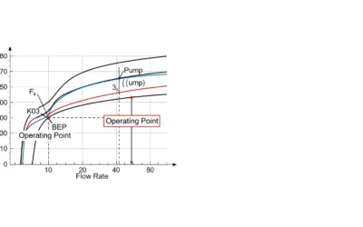
We are looking for the intersection (Operating Point, OP) of the two curves.

Conceptual Intersection

Calculation(s)

We find the intersection by setting \(H_{\text{pump},1} = H_{\text{sys}}\). We will then solve for \(Q\) and finally use that \(Q\) to solve for \(H\).

Step 1: Set equations equal

To find the operating point, we set the pump's supply equal to the system's demand. We use the two equations we just defined in Question 1.

50 - 0.01 \cdot Q^2 = 20 + 0.005 \cdot Q^2

Now we have a single equation with one unknown, \(Q^2\).

Step 2: Isolate \(Q^2\) terms

To solve for \(Q^2\), we group all the constant numbers (50, 20) on the left side and all the terms containing \(Q^2\) on the right side. We do this by subtracting 20 from both sides and adding \(0.01 \cdot Q^2\) to both sides.

\begin{aligned} 50 - 20 &= 0.005 \cdot Q^2 + 0.01 \cdot Q^2 \\ 30 &= (0.005 + 0.01) \cdot Q^2 \\ 30 &= 0.015 \cdot Q^2 \end{aligned}

The equation simplifies to \(30 = 0.015 \cdot Q^2\).

Step 3: Solve for \(Q^2\)

Now, we isolate \(Q^2\) by dividing both sides of the equation by 0.015.

\begin{aligned} Q^2 &= \frac{30}{0.015} \\ &= 2000 \end{aligned}

We find that \(Q^2\) is equal to 2000. We are not done, as this is the flow *squared*.

Step 4: Solve for \(Q\) (Flow)

To find the actual flow \(Q\), we take the square root of \(Q^2\).

\begin{aligned} Q &= \sqrt{2000} \\ &\approx 44.72 \text{ GPM} \end{aligned}

This is the first part of our operating point: the flow rate is 44.72 GPM.

Step 5: Solve for \(H\) (Head)

Now that we have the value for \(Q^2\) (which is 2000), plug it back into *either* original equation to find the corresponding head \(H\). We'll use the system curve equation: \(H_{\text{sys}} = 20 + 0.005 \cdot Q^2\).

\begin{aligned} H &= 20 + 0.005 \cdot (2000) \\ H &= 20 + 10 \\ H &= 30 \text{ ft} \end{aligned}

This is the second part of our operating point: the head is 30 ft. (Note: using the pump curve \(H_{\text{pump},1} = 50 - 0.01 \cdot 2000\) also gives 30 ft, confirming our answer).

Analysis

The single pump will operate at a stable flow of 44.7 GPM, at which point it generates 30 ft of head, exactly matching the 30 ft of head required by the system (20 ft static + 10 ft friction) at that flow rate.

Cautionary Points

A common mistake is to stop after finding \(Q\). The operating point has two coordinates: Flow (\(Q\)) and Head (\(H\)). Always solve for both. You can plug \(Q\) back into *either* equation; you should get the same \(H\). (Try it with the pump curve: \(50 - 0.01 \cdot 2000 = 50 - 20 = 30 \text{ ft}\). It matches!)

Key Takeaways

The operating point is the simultaneous solution to the pump and system equations.
Find it by setting \(H_{\text{pump}} = H_{\text{sys}}\).

Did You Know?

Pump manufacturers also provide a Best Efficiency Point (BEP). This is the flow rate where the pump converts the most electrical energy into water energy. Engineers try to select a pump so that its operating point is as close to its BEP as possible to save energy and prolong the pump's life.

FAQ

[List common follow-up questions students might have.]

Final Result

Single Pump Operating Point: \(Q_1 \approx 44.7 \text{ GPM}\), \(H_1 \approx 30.0 \text{ ft}\).

Your Turn

Using the single pump curve, what head (in ft) would the pump produce if the flow was only 20 GPM?

Memo Card

Question 2 Summary:

Principle: \(H_{\text{pump},1} = H_{\text{sys}}\)
Solution: \(50 - 0.01 \cdot Q^2 = 20 + 0.005 \cdot Q^2\)
Result: \(Q_1 \approx 44.7\) GPM, \(H_1 \approx 30.0\) ft

Question 3: Define Series Pump Curve

Principle

For two identical pumps in series, the combined head at any flow \(Q\) is double the head of a single pump at that same flow \(Q\). The flow must pass through both pumps, so it remains the same, but each pump adds its share of head.

Mini-Lesson

Series vs. Parallel:
- Series (for Head): You add the heads at the same flow rate. \(H_{\text{series}} = H_1 + H_2\). Use this when you need to overcome a large static head or high friction.
- Parallel (for Flow): You add the flows at the same head. \(Q_{\text{parallel}} = Q_1 + Q_2\). Use this when you need to supply a large flow rate to a low-head system.

Pedagogical Note

Think of it like stacking batteries in a flashlight. Putting two 1.5V batteries in series gives you 3.0V (double the "pressure" or head) at the same current (flow). This is the exact same concept.

Formula(s)

We take the single pump equation and multiply the entire expression by 2.

H_{\text{pump},2} = 2 \times H_{\text{pump},1} \] \[ H_{\text{pump},2} = 2 \times (50 - 0.01 \cdot Q^2)

Hypotheses

We assume the pumps are perfectly identical and that there are no additional friction losses from the piping connecting the two pumps.

Data

We use the single pump equation from Q1.

Single Pump Curve: \(H_{\text{pump},1} = 50 - 0.01 \cdot Q^2\)

Tips

Be sure to multiply the *entire* equation by 2. A common mistake is to only multiply the shutoff head (50). You must also multiply the coefficient \(c\), as the "losses" within the pumps are also doubled.

Schematic (Before Calculations)

Graphically, we are "stacking" the pump curves vertically. At any Q, the head H for the new curve is twice as high.

Graphical Addition in Series

Calculation(s)

We apply the principle of adding heads for series pumps (\(H_{\text{pump},2} = 2 \times H_{\text{pump},1}\)). We substitute the full equation for \(H_{\text{pump},1}\) from Question 1.

\begin{aligned} H_{\text{pump},2} &= 2 \times (50 - 0.01 \cdot Q^2) \\ &= (2 \times 50) - (2 \times 0.01) \cdot Q^2 \\ &= 100 - 0.02 \cdot Q^2 \end{aligned}

This new equation, \(H_{\text{pump},2} = 100 - 0.02 \cdot Q^2\), now represents the combined supply curve for both pumps working together in series.

Analysis

This new curve starts at a shutoff head of 100 ft (double the original 50 ft) and has a steeper slope (a coefficient of 0.02 instead of 0.01), reflecting the doubled head contribution at every flow rate.

Cautionary Points

This is for pumps in *series*. Do not confuse this with pumps in *parallel*, where you would solve for \(Q\) in terms of \(H\) and then add the flows (a different, more complex calculation).

Key Takeaways

Pumps in Series: Add Heads at the same Flow.
\(H_{\text{series}} = H_1 + H_2\)

Did You Know?

If the pumps were *different* (e.g., Pump A and Pump B), you would add their unique equations: \(H_{\text{series}} = (H_{0A} - c_A Q^2) + (H_{0B} - c_B Q^2)\). The principle of adding the head equations remains the same.

FAQ

[List common follow-up questions students might have.]

Final Result

Combined Series Curve: \(H_{\text{pump},2} = 100 - 0.02 \cdot Q^2\).

Your Turn

What is the new combined shutoff head (in ft) for the two pumps in series? (This is the head at Q=0).

Memo Card

Question 3 Summary:

Principle: \(H_{\text{pump},2} = 2 \times H_{\text{pump},1}\)
Result: \(H_{\text{pump},2} = 2 \times (50 - 0.01 \cdot Q^2)\)
Final Curve: \(H_{\text{pump},2} = 100 - 0.02 \cdot Q^2\)

Question 4: Calculate Series Operating Point

Principle

We find the new operating point by equating the new combined pump curve (\(H_{\text{pump},2}\)) with the *same* system curve (\(H_{\text{sys}}\)). The system (the piping and elevation) has not changed, but the pump supply has.

Mini-Lesson

Shifting Equilibrium: When you change the "Supply" curve (by adding a pump), the intersection point will "slide" along the *unchanged* "Demand" (system) curve to find a new equilibrium. The new point will be at both a higher flow and a higher head than before.

Pedagogical Note

This is the payoff. We installed a second pump for a reason (presumably, the flow from Q2 was too low). We are now calculating the *actual* new flow rate we will get from this upgrade.

Formula(s)

Set the new pump curve equal to the system curve.

H_{\text{pump},2} = H_{\text{sys}} \] \[ 100 - 0.02 \cdot Q^2 = 20 + 0.005 \cdot Q^2

Hypotheses

We assume the system curve \(H_{\text{sys}} = 20 + 0.005 \cdot Q^2\) is still valid, as the piping has not changed.

Data

We use the system curve from Q1 and the series pump curve from Q3.

System Curve: \(H_{\text{sys}} = 20 + 0.005 \cdot Q^2\)
Series Pump Curve: \(H_{\text{pump},2} = 100 - 0.02 \cdot Q^2\)

Tips

The algebraic process is identical to Question 2, just with different numbers. Again, group constants on one side and \(Q^2\) terms on the other. \(100 - 20 = 0.02 \cdot Q^2 + 0.005 \cdot Q^2\).

Schematic (Before Calculations)

We are looking for the *new* intersection point, which will be higher up on the system curve.

New Operating Point (OP 2)

Calculation(s)

We follow the same process as Question 2, but this time using the new series pump curve, \(H_{\text{pump},2}\).

Step 1: Set equations equal

To find the new operating point, we set the *new* combined pump supply curve (from Q3) equal to the *original* system demand curve (from Q1), which has not changed.

100 - 0.02 \cdot Q^2 = 20 + 0.005 \cdot Q^2

Once again, we have a single equation to solve for \(Q^2\).

Step 2: Isolate \(Q^2\) terms

Just as we did in Question 2, we group the constant terms on the left and the \(Q^2\) terms on the right.

\begin{aligned} 100 - 20 &= 0.005 \cdot Q^2 + 0.02 \cdot Q^2 \\ 80 &= (0.005 + 0.02) \cdot Q^2 \\ 80 &= 0.025 \cdot Q^2 \end{aligned}

The equation simplifies to \(80 = 0.025 \cdot Q^2\).

Step 3: Solve for \(Q^2\)

Now, we isolate \(Q^2\) by dividing both sides of the equation by the new combined coefficient, 0.025.

\begin{aligned} Q^2 &= \frac{80}{0.025} \\ &= 3200 \end{aligned}

We find that \(Q^2\) is 3200. This is the new flow squared value.

Step 4: Solve for \(Q\) (Flow)

We take the square root of 3200 to find the new flow rate \(Q\).

\begin{aligned} Q &= \sqrt{3200} \\ &\approx 56.57 \text{ GPM} \end{aligned}

The new, higher flow rate with two pumps is 56.57 GPM.

Step 5: Solve for \(H\) (Head)

We plug the new \(Q^2\) value (3200) back into the unchanging system curve equation, \(H_{\text{sys}} = 20 + 0.005 \cdot Q^2\), to find the new head.

\begin{aligned} H &= 20 + 0.005 \cdot (3200) \\ H &= 20 + 16 \\ H &= 36 \text{ ft} \end{aligned}

The new operating head is 36 ft. This is higher than the original 30 ft because the higher flow rate causes more friction in the pipes.

Analysis

The new operating point for the two pumps in series is 56.6 GPM at 36 ft. This is a higher flow rate and a higher head than the single pump, which is what we expected.

Cautionary Points

A very common mistake is to think that since the head is doubled, the flow will be doubled. This is false. Doubling the head *supply* does not double the *flow*, because the *system* fights back with more friction (friction is \(\propto Q^2\)).

Key Takeaways

The new operating point is the intersection of the *new* pump curve and the *old* system curve.
The new operating point will be at a higher H and higher Q.

Did You Know?

In a real system, you would also check the pump's "NPSHr" (Net Positive Suction Head Required) against the "NPSHa" (Available) to ensure the pump doesn't cavitate (boil the water) at this new, higher flow rate. Cavitation can quickly destroy a pump.

FAQ

[List common follow-up questions students might have.]

Final Result

Series Operating Point: \(Q_2 \approx 56.6 \text{ GPM}\), \(H_2 \approx 36.0 \text{ ft}\).

Your Turn

Using the system curve, what head (in ft) is required to push 50 GPM through the system?

Memo Card

Question 4 Summary:

Principle: \(H_{\text{pump},2} = H_{\text{sys}}\)
Solution: \(100 - 0.02 \cdot Q^2 = 20 + 0.005 \cdot Q^2\)
Result: \(Q_2 \approx 56.6\) GPM, \(H_2 \approx 36.0\) ft

Question 5: Compare and Analyze Results

Principle

This final step is a synthesis to understand the engineering implications of adding the second pump. We must compare the two operating points to see if the upgrade was effective.

Mini-Lesson

System-Dominated vs. Static-Dominated:
- In a "static-dominated" system (e.g., pumping up a very tall building, \(H_{\text{stat}}\) is high, \(k\) is low), adding a series pump gives a large head increase but small flow increase.
- In a "friction-dominated" system (e.g., a long, flat pipeline, \(H_{\text{stat}}\) is low, \(k\) is high), adding a series pump gives a more balanced increase in both flow and head.

Pedagogical Note

This is the most important question for an engineer. The calculation is done, now you must make a recommendation. Was the cost of a second pump, plus the cost of electricity to run it, worth a 26.6% increase in flow? That depends on the project's goals.

Calculation(s)

We will use the percentage change formula: \(\% \text{ Change} = \frac{\text{New Value} - \text{Old Value}}{\text{Old Value}} \times 100\). We use the rounded values from our results.

Step 1: Calculate % Change in Flow (Q)

We use the flow values from Q2 (Old: 44.7 GPM) and Q4 (New: 56.6 GPM) to find the percentage increase.

\begin{aligned} \% \text{ Change (Flow)} &= \frac{56.6 - 44.7}{44.7} \times 100 \\ &= \frac{11.9}{44.7} \times 100 \\ &= 0.2662 \times 100 \approx +26.6\% \end{aligned}

Adding a second pump in series increased the flow rate by 26.6%.

Step 2: Calculate % Change in Head (H)

Next, we use the head values from Q2 (Old: 30.0 ft) and Q4 (New: 36.0 ft) to find the percentage increase in the operating head.

\begin{aligned} \% \text{ Change (Head)} &= \frac{36.0 - 30.0}{30.0} \times 100 \\ &= \frac{6.0}{30.0} \times 100 \\ &= 0.20 \times 100 = +20.0\% \end{aligned}

The operating head of the system increased by 20.0% to overcome the added friction from the higher flow.

Summary Table

This confirms the values in the table.

Parameter	Single Pump (from Q2)	Two Pumps in Series (from Q4)	% Change
Flow (Q)	44.7 GPM	56.6 GPM	+26.6%
Head (H)	30.0 ft	36.0 ft	+20.0%

Schematic (After Calculations)

The best visual summary is the final chart from the simulator, which shows both operating points on the same graph.

Analysis

Adding a second pump in series did not double the flow. It didn't even come close. It provided a moderate increase in flow (+26.6%) while overcoming the much higher friction (+20% head). This confirms the rule: pumps are added in series to overcome higher heads. If the goal was to *double the flow*, the correct choice would have been pumps in parallel (and likely larger pipes to reduce friction).

Cautionary Points

Never assume linear returns. Doubling the pumps does not double the performance. The system curve *always* dictates the final operating point, and its quadratic nature provides "diminishing returns" on pump upgrades.

Key Takeaways

Series pumps are for "high head" applications.
The gain in flow is limited by the steepness of the system curve (friction).
Always analyze the *new* operating point; don't just add pump specs.

Did You Know?

In long-distance oil and gas pipelines, "booster stations" (which are just large pumps in series) are placed every 50-100 miles. Their sole purpose is to add pressure (head) back into the line to overcome the friction losses from the previous section, keeping the flow rate constant.

FAQ

[List common follow-up questions students might have.]

Final Result

The series configuration successfully boosted the system's flow to 56.6 GPM and head to 36 ft, overcoming the increased friction.

Your Turn

What was the percentage increase in flow? (e.g., 26.6)

Memo Card

Question 5 Summary:

Result 1 (1 Pump): \(Q_1 \approx 44.7\) GPM, \(H_1 \approx 30.0\) ft
Result 2 (2 Pumps): \(Q_2 \approx 56.6\) GPM, \(H_2 \approx 36.0\) ft
Conclusion: Flow increased by 26.6%, not 100%.

Interactive Tool: System & Pump Curve Simulator

Use the sliders to change the system's static head and friction coefficient. See how it changes the operating point for both a single pump and two pumps in series.

Input Parameters

Static Head (\(H_{\text{stat}}\)) [ft] 20 ft

Friction Coefficient (\(k\)) [ft/GPM²] 0.005 ft/GPM²

Calculated Operating Points

Single Pump Flow (Q) - GPM

Series Pump Flow (Q) - GPM

Final Quiz: Test Your Knowledge

1. Generally, pumps are installed in series to...

Increase the total head (pressure) in the system.
Increase the total flow rate in the system.
Decrease the system's friction losses.

2. The System Curve is a function of...

The pump's motor speed only.
The static head only.
The static head plus the friction losses (which depend on flow).

3. The "Operating Point" of a pump is...

The point of maximum efficiency on the pump curve.
Where the pump curve intersects the system curve.
The shutoff head of the pump.

Glossary

Operating Point: The specific flow rate (Q) and head (H) where the pump's performance curve intersects the hydraulic system's resistance curve. This is the stable point at which the system will operate.
System Curve: A graphical representation of the total head required to move fluid through a piping system at various flow rates. It is the sum of static head and all friction losses. \(H_{\text{sys}} = H_{\text{static}} + H_{\text{friction}}\).
Pump Characteristic Curve: A graph provided by a pump manufacturer that shows the pump's performance, typically plotting head, efficiency, and NPSHr against a range of flow rates.
Static Head: The vertical difference in elevation between the source fluid level and the discharge fluid level, independent of flow. \(H_{\text{stat}} = \text{WL}_{\text{discharge}} - \text{WL}_{\text{suction}}\).
Pumps in Series: A configuration where the discharge of one pump is connected to the suction of the next. This setup is used to add the head of each pump, achieving a higher total pressure.