Analysis of Temperature Effects in Hydraulics
Context: The Impact of Thermal Variations on Hydraulic Systems.
In many industrial applications, from petrochemicals to HVAC, fluids are transported at widely varying temperatures. Temperature has a direct and significant effect on a fluid's physical properties, especially its viscosityViscosity measures a fluid's resistance to flow. A highly viscous fluid (like honey) flows with difficulty, while a low-viscosity fluid (like water) flows easily. and density. These changes can considerably alter a network's performance, particularly by modifying head loss and the required pumping power.
Pedagogical Note: This exercise will teach you how to quantify the impact of a temperature change on linear head loss in a pipe, an essential skill for designing and optimizing hydraulic networks.
Learning Objectives
- Understand the influence of temperature on water's viscosity and density.
- Calculate the Reynolds number and determine the flow regime at different temperatures.
- Apply the iterative Colebrook-White method to accurately determine the head loss coefficient.
- Quantify the variation in linear head loss due to an increase in temperature.
Study Data
Technical Data
| Characteristic | Value |
|---|---|
| Pipe Material | Cast Iron |
| Absolute Roughness (\(\epsilon\)) | 0.00177 in (0.045 mm) |
| Fluid | Water |
Physical Properties of Water
| Property | Value at 41°F (5°C) | Value at 95°F (35°C) |
|---|---|---|
| Density (\(\rho\)) | 1000 kg/m³ | 994 kg/m³ |
| Dynamic Viscosity (\(\mu\)) | \(1.519 \times 10^{-3}\) Pa·s | \(0.723 \times 10^{-3}\) Pa·s |
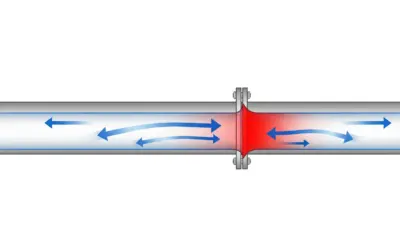
Pipe Section Diagram
| Operating Parameter | Symbol | Value (USCU) | Value (SI) |
|---|---|---|---|
| Internal Diameter | \(D\) | 5.91 in | (150 mm) |
| Pipe Length | \(L\) | 1640.4 ft | (500 m) |
| Volumetric Flow Rate | \(Q\) | ~440.3 GPM | (100 m³/h) |
Questions to Solve
- Winter Case: Calculate the linear head loss (in feet and meters of water column) for water at 41°F (5°C).
- Summer Case: Calculate the linear head loss (in feet and meters of water column) for water at 95°F (35°C).
- Compare the two results and conclude on the effect of temperature on the required pumping energy.
Fundamentals of Fluid Mechanics
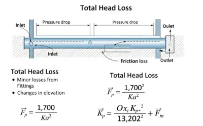
To solve this exercise, it's essential to master the concept of head loss, which represents the energy "lost" by a fluid in motion due to friction against the pipe walls.
1. Fluid Properties and Temperature
For a liquid like water, an increase in temperature leads to a decrease in its density (\(\rho\)) and, most importantly, a sharp decrease in its dynamic viscosity (\(\mu\)). This latter point has the greatest influence on friction.
2. Linear Head Loss (Darcy-Weisbach)
The energy loss due to friction over the length of a pipe is calculated using the Darcy-Weisbach equation:
\[ \Delta h = \lambda \cdot \frac{L}{D} \cdot \frac{v^2}{2g} \]
Where \(\Delta h\) is the head loss (in m or ft), \(\lambda\) is the dimensionless head loss coefficient, \(L\) is the length, \(D\) is the diameter, \(v\) is the velocity, and \(g\) is the acceleration due to gravity.
3. Head Loss Coefficient (Colebrook-White Equation)
The value of \(\lambda\) depends on the flow regime (characterized by the Reynolds numberA dimensionless number that characterizes a fluid's flow regime. A low Re indicates laminar (smooth) flow, while a high Re indicates turbulent (chaotic) flow., \(Re\)) and the relative roughness of the pipe (\(\epsilon/D\)). For turbulent flow (\(Re > 4000\)), the standard is the implicit Colebrook-White equation, which requires an iterative solution:
\[ \frac{1}{\sqrt{\lambda}} = -2 \log_{10} \left( \frac{\epsilon/D}{3.7} + \frac{2.51}{Re \sqrt{\lambda}} \right) \]
Solution: Analysis of Temperature Effects in Hydraulics
Question 1: Head Loss Calculation at 41°F (5°C)
Principle
The physical concept is that a flowing fluid's energy dissipates as heat due to friction with the pipe wall. This energy loss, called head loss, depends on the fluid's velocity, the pipe's dimensions, and the fluid's properties (viscosity, density), which are themselves influenced by temperature.
Mini-Lesson
Linear head loss is a direct consequence of the shear stress exerted by the fluid on the wall. In a turbulent regime, this exchange is dominated by eddies and chaotic fluid motion. Viscosity plays a key role by dampening these eddies near the wall, in what is known as the viscous sublayer.
Pedagogical Note
The key is to follow a logical process: geometric characteristics → fluid properties for the given T° → velocity → Reynolds number → friction coefficient \(\lambda\) → head loss. Each step follows from the previous one. Don't jump to the final calculation without validating each intermediate step.
Standards
This exercise uses recognized academic formulas. In a professional context, engineers might use simulation software (like AFT Fathom or Pipe-Flo) that integrates these calculations and fluid databases compliant with standards (e.g., ASME, API).
Formula(s)
Velocity Formula
Reynolds Number Formula
Colebrook-White Formula (Implicit)
Darcy-Weisbach Formula
Assumptions
For this calculation, we make the following simplifying assumptions:
- The flow is steady (constant flow rate).
- The fluid is incompressible (density is constant along the pipe).
- The pipe is full, and the velocity profile is fully developed.
- The temperature is uniform throughout the fluid and constant over the studied length.
Given Data (in SI units)
We use the problem data and the physical properties of water at 5°C. All calculations will be performed in SI units for consistency (as the JS logic relies on them). USCU equivalents are for reference.
| Parameter | Symbol | Value (SI) | Value (USCU) |
|---|---|---|---|
| Density (5°C) | \(\rho\) | 1000 | kg/m³ |
| Dynamic Viscosity (5°C) | \(\mu\) | \(1.519 \times 10^{-3}\) | Pa·s |
| Diameter | D | 0.15 | m |
| Length | L | 500 | m |
| Flow Rate | Q | 0.0278 | m³/s |
| Roughness | \(\epsilon\) | \(4.5 \times 10^{-5}\) | m |
Tips
To start the iterative Colebrook-White calculation, you need an initial guess for \(\lambda\). You can use an explicit formula like Haaland's to get a starting value very close to the final solution, which speeds up convergence.
Diagram (Before Calculations)
Pipe Model
Calculation(s)
Step 1: Unit Conversions
To ensure consistent calculations, all values must be in SI units (meters, seconds, kg, etc.).
Flow Rate (Q) Conversion
The flow rate is now in cubic meters per second. (Flow rate is ~440.3 GPM or 0.982 cfs).
Diameter (D) Conversion
The diameter is converted to meters. (Diameter is ~0.492 ft).
Roughness (\(\epsilon\)) Conversion
The roughness is also converted to meters. (Roughness is ~1.48e-4 ft).
Step 2: Base Parameter Calculation
Cross-Sectional Area (A) Calculation
This is the available flow area inside the pipe. (Approx. 0.190 sq ft).
Velocity (v) Calculation
The average fluid velocity in the pipe is 1.57 m/s. (Approx. 5.15 ft/s).
Reynolds Number (Re) Calculation
The Reynolds number is 155,036. Since this is much greater than 4,000, the flow is confirmed to be turbulent.
Relative Roughness Calculation
This dimensionless ratio quantifies the pipe's "roughness" relative to its size. It is needed for the Colebrook equation.
Step 3: Iterative Calculation of Friction Factor (\(\lambda\))
We start with a guess, e.g., \(\lambda_0 \approx 0.0166\).
Iteration 1
Our first calculated estimate is \(\lambda_1 \approx 0.0184\). We reuse this value for the next iteration.
Iteration 2
The result (\(\lambda_2 \approx 0.0183\)) is very close to the previous one (\(\lambda_1 \approx 0.0184\)). The value has converged. We will use \(\lambda = 0.0183\).
Step 4: Final Head Loss (\(\Delta h\)) Calculation
Now that we have all components ( \(\lambda\), L, D, v, g), we can calculate the final head loss.
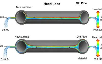
The final result is a head loss of 25.13 feet (7.66 meters) for water at 41°F.
Diagram (After Calculations)
Head Loss Visualization
Reflections
A result of 25.13 ft means that over 1640 ft, the fluid lost an amount of energy equivalent to falling from a height of 25.13 feet. This energy, converted to heat, must be supplied by an upstream pump to maintain the flow.
Points of Caution
The most common error is forgetting unit conversions. While USCU units are common, most core fluid dynamics formulas (like Reynolds number with Pa·s) are derived for SI units. Always convert to a consistent system (like SI) for calculation, then convert the final answer back.
Key Takeaways
For a given pipe and flow rate, calculating linear head loss comes down to correctly determining the friction factor \(\lambda\), which is a direct function of the fluid properties (via \(Re\)) and the pipe's surface condition (via \(\epsilon/D\)).
Did You Know?
The Moody diagram, a graphical representation of the Colebrook-White equation, was published in 1944 by Lewis Ferry Moody (an American engineer) and remains an essential reference for hydraulic engineers worldwide.
FAQ
It's normal to have questions.
Final Result
Try It Yourself
If the flow rate were reduced to 75 m³/h in winter (41°F), what would be the new head loss in feet?
Question 2: Head Loss Calculation at 95°F (35°C)
Principle
The physical principle is the same as in Question 1. However, we will now see how a change in temperature, by modifying the fluid's properties (especially its viscosity), impacts the flow's turbulence (via the Reynolds number) and, consequently, the friction and final energy loss.
Mini-Lesson
The thermal agitation of a liquid's molecules reduces the intermolecular cohesive forces. This is why, when a liquid like water is heated, its viscosity decreases: the molecules "slide" past each other more easily. Less viscosity means less energy dissipation through internal friction, which affects the overall flow.
Pedagogical Note
Here, the only thing that changes from Question 1 is the fluid properties. This is an excellent exercise for isolating the impact of a single parameter. Be meticulous: do not reuse the Reynolds number or \(\lambda\) from the previous question! Each case must be recalculated.
Standards
Data on water properties as a function of temperature come from standardized tables, such as those from IAPWS (International Association for the Properties of Water and Steam), which are global references for engineers.
Formula(s)
Velocity Formula
Reynolds Number Formula
Colebrook-White Formula (Implicit)
Darcy-Weisbach Formula
Assumptions
The assumptions are identical to those in the first question (steady flow, incompressible fluid, full pipe, etc.).
Given Data (in SI units)
We use the geometric and flow data from the problem, along with the properties of water at 35°C.
| Parameter | Symbol | Value (SI) | Unit |
|---|---|---|---|
| Density (35°C) | \(\rho\) | 994 | kg/m³ |
| Dynamic Viscosity (35°C) | \(\mu\) | \(0.723 \times 10^{-3}\) | Pa·s |
| Diameter | D | 0.15 | m |
| Length | L | 500 | m |
| Flow Rate | Q | 0.0278 | m³/s |
| Roughness | \(\epsilon\) | \(4.5 \times 10^{-5}\) | m |
Tips
Since the viscosity decreases sharply, expect a significantly larger Reynolds number. This will push the flow closer to the "fully rough turbulent" regime, where \(\lambda\) becomes less sensitive to changes in Reynolds number. The final result for \(\lambda\) should therefore be slightly lower than in Q1, but not radically different.
Diagram (Before Calculations)
Pipe Model
Calculation(s)
Geometric parameters, flow rate, and velocity do not change: \(v \approx 1.57\,\text{m/s}\) and \(\epsilon/D = 0.0003\). We recalculate the temperature-dependent parameters.
Step 1: Reynolds Number (Re) Calculation
We use the new values for density (\(\rho = 994\)) and viscosity (\(\mu = 0.723 \times 10^{-3}\)).
At 35°C, the Reynolds number (323,788) is much higher than at 5°C (155,036) because the viscosity has dropped. The flow is even more turbulent.
Step 2: Iterative Calculation of Friction Factor (\(\lambda\))
We start with a guess, e.g., \(\lambda_0 \approx 0.0146\).
Iteration 1
The first calculated estimate is \(\lambda_1 \approx 0.0170\).
Iteration 2
The new value is \(\lambda_2 \approx 0.0168\).
Iteration 3
The result \(\lambda_3 \approx 0.0169\) is almost identical to \(\lambda_2 \approx 0.0168\). The value has converged. We will use \(\lambda \approx 0.0169\).
Step 3: Final Head Loss (\(\Delta h\)) Calculation
We use this new friction factor \(\lambda\) for the final calculation.
The head loss at 95°F is 23.20 feet (7.07 meters). This is lower than the value calculated at 41°F.
Diagram (After Calculations)
Head Loss Visualization (95°F)
Reflections
The increase in the Reynolds number from 155,036 to 323,788 is dramatic. It shows how much more turbulent the flow becomes (inertial forces become even more dominant). This "flattens" the velocity profile and reduces the thickness of the viscous sublayer, slightly decreasing the relative influence of friction, hence the drop in \(\lambda\).
Points of Caution
Don't hastily conclude that a large increase in Reynolds number will always lead to a large drop in \(\lambda\). In the fully rough turbulent zone of the Moody diagram, the curve for \(\lambda\) becomes nearly horizontal: the friction factor then depends almost exclusively on the relative roughness.
Key Takeaways
Higher temperatures make water "thinner" (less viscous). For the same flow rate, this results in more turbulent flow (higher Re) and slightly lower friction losses.
Did You Know?
In cooling systems for nuclear reactors, precise control over water properties at high temperature and pressure is absolutely critical. Extremely complex thermodynamic models are used to predict its behavior and ensure safety.
FAQ
Final Result
Try It Yourself
What would the head loss (in feet) be at 95°F (35°C) if the pipe were smooth PVC (\(\epsilon \approx 0.0015\,\text{mm}\))?
Question 3: Comparison and Conclusion
Principle
The goal is to synthesize the previous results to draw a practical engineering conclusion. It's no longer just about calculating, but about analyzing a trend and quantifying its importance to assess whether the effect of temperature is a negligible factor or a parameter to be considered in the system's design and operation.
Mini-Lesson
Sensitivity analysis is a fundamental process in engineering. It involves studying how the variation of an input parameter (here, temperature) affects an output result (head loss). This helps identify the most influential parameters and optimize a system's design.
Pedagogical Note
A good conclusion isn't just "it's smaller" or "it's bigger." It must be quantified. Always calculate the variation in both absolute and percentage terms. This provides a much more meaningful order of magnitude for an engineer or decision-maker.
Standards
In energy balances or facility audits (like the ISO 50001 standard for energy management), such analyses are crucial for identifying potential energy savings. The impact of temperature on pumping would be a typical point of study.
Formula(s)
Relative Change Formula
Assumptions
We assume the pump and its motor have a constant efficiency, although in reality, the pump's operating point on its characteristic curve might slightly shift with the change in the system's head loss.
Data
We use the final results from the two previous questions.
| Condition | Symbol | Value (USCU) | Value (SI) |
|---|---|---|---|
| Head Loss (Winter, 41°F) | \(\Delta h_{5^\circ\text{C}}\) | 25.13 ft | (7.66 m) |
| Head Loss (Summer, 95°F) | \(\Delta h_{35^\circ\text{C}}\) | 23.20 ft | (7.07 m) |
Astuces
No calculation tips here; the analysis is what matters.
Diagram (Before Calculations)
Head Loss Comparison
Calculation(s)
Absolute Change Calculation
We subtract the new head loss (summer) from the original (winter).
The head loss decreased by 1.93 feet (0.59 meters).
Relative Change Calculation
We calculate this decrease as a percentage of the initial (winter) value. The ratio is the same regardless of units.
This represents a 7.7% decrease in head loss as the water warms from 41°F to 95°F.
Diagram (After Calculations)
Head Loss Comparison
Reflections
A 7.7% reduction in head loss means the pump must provide 7.7% less energy to overcome friction. Since hydraulic power is proportional to head loss (\(P_{\text{hyd}} = Q \cdot \rho \cdot g \cdot \Delta h\)), the pump's electrical consumption will decrease by a similar proportion (depending on efficiency). Over a year, for a multi-kilowatt pump running continuously, the savings could be in the hundreds or even thousands of dollars.
Points of Caution
Do not generalize this result to all fluids! For gases, an increase in temperature *increases* viscosity, which would have the opposite effect: head loss would increase! This analysis is valid only for liquids.
Key Takeaways
Key Takeaway: For a constant flow rate in a given network, an increase in the temperature of water (or most liquids) causes a decrease in its viscosity. This increases the Reynolds number and decreases the friction factor \(\lambda\), resulting in a reduction in head loss and therefore lower energy consumption for the pump.
Did You Know?
This phenomenon is crucial in oil pipelines transporting crude oil. Oil can be very viscous at low temperatures. It is therefore heated to reduce its viscosity and facilitate its transport over thousands of miles, drastically reducing pumping costs.
FAQ
Final Result
Try It Yourself
No interactive exercise for this summary question.
Interactive Tool: Thermal Impact Simulator
Use the sliders to vary the water temperature and flow rate in the exercise's pipe. Observe the real-time impact on the Reynolds number, friction factor, and total head loss.
Input Parameters
Key Results
Final Quiz: Test Your Knowledge
1. What generally happens to the dynamic viscosity of water as its temperature increases?
2. A higher Reynolds number indicates...
3. In the Darcy-Weisbach formula, the friction factor \(\lambda\) primarily depends on:
4. If the water temperature in a pipe increases while the flow rate remains constant, the linear head loss will:
5. Which fluid property is the main cause of this change in head loss with temperature?
Glossary
- Head Loss
- Energy dissipated by a fluid in motion, typically due to friction against pipe walls (linear loss) or passing through fittings like valves and elbows (singular loss). It is measured in Pascals (pressure) or meters/feet of fluid column (height).
- Dynamic Viscosity (\(\mu\))
- A fluid's property that measures its internal resistance to flow. It is often expressed in Pascal-seconds (Pa·s). The higher the viscosity, the "thicker" the fluid and the more it resists motion.
- Reynolds Number (\(Re\))
- A dimensionless number used in fluid mechanics to characterize a flow regime. It represents the ratio of inertial forces to viscous forces. \(Re < 2000\) typically indicates laminar (orderly) flow, while \(Re > 4000\) indicates turbulent (chaotic) flow.
- Roughness (\(\epsilon\))
- A measure of the texture of a pipe's inner surface. High roughness increases friction and thus increases head loss.


0 Comments