EGL and HGL Calculation

Exercise: EGL and HGL Calculation

Calculating the Energy Grade Line (EGL) and Hydraulic Grade Line (HGL)

Context: The study of pressurized pipe flowFlow of a fluid that completely fills a closed conduit. The pressure can be greater or less than atmospheric pressure..

Understanding the distribution of energy in a hydraulic network is fundamental for any engineer. This exercise focuses on determining and visualizing this energy through two key concepts: the Energy Grade Line (EGL) and the Hydraulic Grade Line (HGL). We will analyze a practical case of water flowing between two reservoirs through a pipe of varying diameter to understand how geometry and friction influence the fluid's pressure and total energy.

Pedagogical Note: This exercise will teach you to apply the general Bernoulli's equation to a real case including head losses, conduct an iterative calculation to find the flow rate, and interpret the energy behavior of a flow.

Learning Objectives

Apply the generalized Bernoulli's equation to a pipe system.
Calculate friction losses (major) and minor losses.
Determine the flow rate in a pipe using an iterative method.
Plot and interpret the Energy Grade Line (EGL) and Hydraulic Grade Line (HGL) of a flow.

Problem Data

A steel pipe connects two large reservoirs, A and B. Water flows from A to B by gravity. The pipe consists of two straight sections with different diameters. Minor losses at the elbow connecting the two sections are considered negligible.

Schematic of the Hydraulic System

Parameter	Symbol	Value	Unit
Elevation, Reservoir A	$ z_A $	300	$\text{ft}$
Elevation, Reservoir B	$ z_B $	270	$\text{ft}$
Length / Diameter Section 1	$ L_1 \ / \ D_1 $	1600 / 8	$\text{ft / in}$
Length / Diameter Section 2	$ L_2 \ / \ D_2 $	1000 / 6	$\text{ft / in}$
Pipe Roughness (steel)	$ \epsilon $	0.00033	$\text{ft}$
Kinematic Viscosity of Water	$ \nu $	$1.08 \times 10^{-5}$	$\text{ft}^2/\text{s}$

Questions to Solve

Write the generalized Bernoulli's equation (Energy Equation) between the free surfaces of reservoirs A and B.
Express the total head loss $ h_L $ as a function of the velocities $ V_1 $ and $ V_2 $ in the two sections. Account for minor losses: entrance ($K_e=0.5$), sudden contraction ($K_c=0.2$), and exit ($K_s=1.0$).
Using the continuity equation, express $ V_2 $ as a function of $ V_1 $.
Using an iterative method (2 iterations will suffice), determine the velocities $ V_1 $, $ V_2 $, and the volumetric flow rate $ Q_v $.
Calculate the total head and piezometric head at key points (entrance, junction, exit) and sketch the Energy Grade Line (EGL) and Hydraulic Grade Line (HGL).

Fundamentals of Pipe Flow

To solve this exercise, two fundamental principles of fluid mechanics are necessary: the conservation of energy and the evaluation of energy losses due to friction.

1. Generalized Bernoulli's Equation (Energy Equation)
This theorem is an expression of the conservation of energy for a moving fluid. It states that between two points on a streamline, the total head (energy per unit weight) at the upstream point is equal to the total head at the downstream point, plus the head losses between the two points. \[ z_1 + \frac{P_1}{\gamma} + \frac{V_1^2}{2g} = z_2 + \frac{P_2}{\gamma} + \frac{V_2^2}{2g} + h_{L, 1 \to 2} \] Where $ z $ is the elevation, $ P $ is the pressure, $ \gamma = \rho g $ is the specific weight, $ V $ is the velocity, and $ h_L $ is the total head loss.

2. Friction Losses (Darcy-Weisbach)
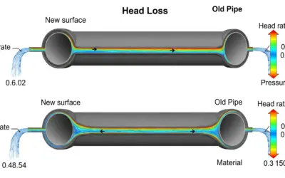
Energy is dissipated by friction along a pipe. This "major" or "friction" loss is calculated by the Darcy-Weisbach equation: \[ h_f = f \frac{L}{D} \frac{V^2}{2g} \] The friction factor $ f $ (note: $f = 4 \times f_{\text{Fanning}}$) depends on the Reynolds NumberA dimensionless number that characterizes the flow regime (laminar or turbulent). $ Re = \frac{VD}{\nu} $ and the relative roughness $ \epsilon/D $. It is often determined using the (implicit) Colebrook-White equation or the Moody diagram.

Solution: EGL and HGL Calculation

Question 1: The Energy Equation

Principle

We apply the principle of energy conservation between the two points where the energy is easiest to define: the free surfaces of the reservoirs. At these points, the pressure is atmospheric, and the velocity is considered zero, which simplifies the energy balance.

Mini-Course

Bernoulli's equation is a cornerstone of fluid mechanics. The "generalized" version (or Energy Equation) is essential in engineering because it accounts for the energy losses (head losses) that inevitably occur in real systems.

Pedagogical Note

The trick here is to always choose start and end points for which you have the most information. The free surfaces of large reservoirs are ideal because the pressure is known (atmospheric) and the velocity is zero, which greatly simplifies the equation.

Standards

While this is an academic exercise, the Energy Equation is a foundation of fluid mechanics taught in all engineering curricula. Hydraulic network calculations are systematically based on this theorem.

Formula(s)

Generalized Bernoulli's Equation

z_A + \frac{P_A}{\gamma} + \frac{V_A^2}{2g} = z_B + \frac{P_B}{\gamma} + \frac{V_B^2}{2g} + h_{L, A \to B}

Assumptions

We simplify the equation by making the following assumptions for large reservoirs open to the atmosphere:

The pressure at the free surfaces is atmospheric pressure. In gage pressure, we set $ P_A = P_B = 0 $.
The velocities at the free surfaces are negligible: $ V_A \approx 0 $ and $ V_B \approx 0 $.

Data

The only data needed for this first question are the elevations of the free surfaces.

Parameter	Symbol	Value	Unit
Elevation Reservoir A	$z_A$	300	$\text{ft}$
Elevation Reservoir B	$z_B$	270	$\text{ft}$

Tips

To avoid errors, always think in terms of an "energy balance." The energy available at the start (head at A) must equal the energy remaining at the end (head at B) plus all the energy "lost" along the way (head losses).

Schematic (Before calculation)

Schematic of the Hydraulic System

Calculation(s)

We start with the full energy equation:

z_A + \frac{P_A}{\gamma} + \frac{V_A^2}{2g} = z_B + \frac{P_B}{\gamma} + \frac{V_B^2}{2g} + h_{L, A \to B}

Now, we simplify by applying our assumptions (gage pressures $P_A, P_B = 0$ and velocities $V_A, V_B = 0$) :

z_A + 0 + 0 = z_B + 0 + 0 + h_{L, A \to B}

The equation is now greatly simplified. We just need to isolate the total head loss $ h_{L, A \to B} $ and substitute the elevation values:

\begin{aligned} h_{L, A \to B} &= z_A - z_B \\ &= 300 \text{ ft} - 270 \text{ ft} \\ &= 30 \text{ ft} \end{aligned}

This result is the net elevation drop, or "static head." It means that all the potential energy from the 30 ft height difference will be dissipated by head losses in the pipe.

Schematic (After calculation)

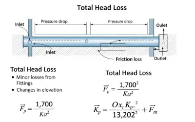
Visualization of Total Head Loss

Reflections

This result is fundamental: it means the only "driving force" for the flow is the 30 ft elevation difference between the two reservoirs. All this gravitational potential energy will be dissipated by friction and minor losses in the pipe.

Points of Caution

Be careful not to confuse head (an elevation, in feet) with pressure (in psi). Remember that for free surfaces, the *gage* pressure is zero, but the absolute pressure is atmospheric pressure.

Key Takeaways

The driver for gravity-fed flow is the difference in total head between the start and end points.
For reservoirs, this total head is simply their surface elevation.

Did you know?

Daniel Bernoulli, an 18th-century Swiss mathematician and physicist, formulated this fundamental principle without being able to account for head losses. It wasn't until the 19th century that engineers like Darcy and Weisbach completed his work to apply it to real-world cases.

FAQ

It's normal to have questions.

Final Result

The total head loss between the two reservoirs must be equal to the elevation drop: $ h_L = 30 \text{ ft} $.

Your Turn

If reservoir B was at an elevation of 250 ft, what would the total head loss be?

Question 2: Total Head Loss Expression

Principle

The total head loss ($h_L$) is the sum of all energy losses experienced by the fluid along its path. We distinguish between friction losses (or major losses, $h_f$, due to friction over the length) and minor losses ($h_m$, due to fittings, bends, and transitions).

Mini-Course

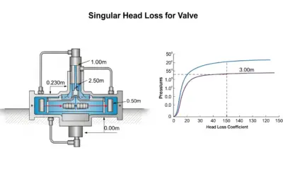
Minor losses are caused by the turbulence generated when the fluid passes through a component (bend, valve, etc.). They are generally proportional to the fluid's kinetic energy ($V^2/2g$). The proportionality constant K is called the minor loss coefficient and depends on the component's geometry.

Pedagogical Note

A common mistake is to forget one of the minor losses. You must mentally "follow" a particle of fluid from start to finish and list every "obstacle" it encounters: the entrance, section changes, valves, bends, and the exit.

Standards

The values of minor loss coefficients (K) are tabulated in many hydraulic reference manuals, such as those by Idelcik, Miller, or the Crane Technical Paper 410. These values are derived from laboratory experiments.

Formula(s)

Total Head Loss Breakdown

h_L = h_{f,1} + h_{f,2} + h_m

Minor Loss Breakdown

h_m = h_{m,\text{entry}} + h_{m,\text{contraction}} + h_{m,\text{exit}}

Head Loss Formulas

h_f = f \frac{L}{D} \frac{V^2}{2g} \quad ; \quad h_m = K \frac{V^2}{2g}

Assumptions

We assume the given K coefficients are constant and do not depend on the Reynolds number, which is a common assumption for turbulent flow.

Data

We use the geometric data for the pipe and the minor loss coefficients.

Parameter	Symbol	Value	Unit
Pipe 1 Data	$L_1, D_1$	1600, 8	$\text{ft, in}$
Pipe 2 Data	$L_2, D_2$	1000, 6	$\text{ft, in}$
Entrance Coefficient	$K_e$	0.5	-
Contraction Coefficient	$K_c$	0.2	-
Exit Coefficient	$K_s$	1.0	-

Tips

For minor losses, pay close attention to the reference velocity. By convention, for a contraction or expansion, the velocity in the *downstream* section (usually the faster one) is used, but this problem specifies using $V_2$ for the contraction, which is standard.

Schematic (Before calculation)

Identification of Head Loss Locations

Calculation(s)

We sum all the head losses identified, grouping them by type:

Friction (Major) Losses: $ h_{f,1} + h_{f,2} $
Minor Losses: $ h_{m,\text{entry}} + h_{m,\text{contraction}} + h_{m,\text{exit}} $

Now, we replace each term with its formula (Darcy-Weisbach for friction, $K \cdot V^2/2g$ for minor). The first line is the conceptual sum, the second is the substitution, and the third groups the terms by velocity ($V_1$ or $V_2$) :

\begin{aligned} h_L &= h_{f,1} + h_{f,2} + h_{m,\text{entry}} + h_{m,\text{contr.}} + h_{m,\text{exit}} \\ &= \left(f_1 \frac{L_1}{D_1} \frac{V_1^2}{2g}\right) + \left(f_2 \frac{L_2}{D_2} \frac{V_2^2}{2g}\right) + \left(K_e \frac{V_1^2}{2g}\right) + \left(K_c \frac{V_2^2}{2g}\right) + \left(K_s \frac{V_2^2}{2g}\right) \\ &= \frac{V_1^2}{2g} \left( f_1 \frac{L_1}{D_1} + K_e \right) + \frac{V_2^2}{2g} \left( f_2 \frac{L_2}{D_2} + K_c + K_s \right) \end{aligned}

This final equation is our working model. It links the total head loss (which we know, 30 ft) to the two unknown velocities ($V_1$ and $V_2$) and the friction factors ($f_1$ and $f_2$), which we also don't know yet.

Schematic (After calculation)

Conceptual Breakdown of Total Head Loss

Reflections

This equation shows how each component of the system (length, diameter, fittings) contributes to the total energy dissipation. Notice that the losses are proportional to the square of the velocities, meaning they increase very rapidly with flow rate.

Points of Caution

Be sure to associate each head loss with the correct velocity: losses in section 1 depend on $V_1$, those in section 2 depend on $V_2$. The entrance loss depends on $V_1$, while the contraction and exit losses depend on $V_2$.

Key Takeaways

Total head loss is the sum of friction (major) losses and minor losses.
Each type of loss is expressed in terms of the velocity head, $V^2/2g$.

Did you know?

In long pipelines, friction losses often account for over 95% of the total losses, and minor losses can sometimes be neglected. Conversely, in compact systems (like building plumbing), minor losses from elbows and tees can be dominant.

FAQ

It's normal to have questions.

Final Result

The final expression, grouping terms by velocity, is:
\[ h_L = \frac{V_1^2}{2g} \left( f_1 \frac{L_1}{D_1} + K_e \right) + \frac{V_2^2}{2g} \left( f_2 \frac{L_2}{D_2} + K_c + K_s \right) \]

Your Turn

If we added a half-open gate valve ($K_v=2.5$) in Section 1, how would the final result equation change?

The term in $V_1^2/2g$ would become $(f_1 \frac{L_1}{D_1} + K_e + 2.5)$.

Question 3: Velocity Relationship

Principle

The continuity equation expresses the conservation of mass for an incompressible fluid. For a constant flow rate, the product of the velocity and the cross-sectional area is constant. If the area decreases, the velocity must increase, and vice-versa.

Mini-Course

For an incompressible fluid (constant density), mass conservation implies volumetric flow rate conservation ($Q_v$). The flow rate is the volume of fluid passing through a section per unit time, and it equals the product of the cross-sectional area $A$ and the average fluid velocity $V$ through that section: $Q_v = A \cdot V$.

Pedagogical Note

This is a crucial simplification step. By relating $V_2$ to $V_1$, we can express the total head loss in terms of a single unknown velocity, $V_1$, which makes the energy equation solvable.

Standards

The principle of mass conservation, along with conservation of energy and momentum, is one of the three fundamental pillars upon which all of fluid mechanics is built.

Formula(s)

Continuity Equation

\[ Q_v = A_1 V_1 = A_2 V_2 \]

where $ A = \frac{\pi D^2}{4} $ is the area of the circular section.

Assumptions

We assume the fluid (water) is incompressible, which is an excellent approximation for liquids in most common applications.

Data

The only data needed are the diameters of the two sections.

Parameter	Symbol	Value	Unit
Diameter Section 1	$D_1$	8	$\text{in}$
Diameter Section 2	$D_2$	6	$\text{in}$

Tips

When calculating the velocity ratio, you don't need to convert the diameters to feet, as the ratio $D_1/D_2$ is dimensionless. Just make sure they are in the same unit (here, inches).

Schematic (Before calculation)

Visualization of Flow Rate Conservation

Calculation(s)

We set the flow rates equal (mass conservation), solve for $V_2$ in terms of $V_1$, and replace the areas with their formulas in terms of diameter, $ A = \pi D^2 / 4 $. The $\pi/4$ terms cancel out:

\begin{aligned} Q_v &= A_1 V_1 = A_2 V_2 \\ V_2 &= V_1 \frac{A_1}{A_2} \\ &= V_1 \frac{\pi D_1^2 / 4}{\pi D_2^2 / 4} \\ &= V_1 \left( \frac{D_1}{D_2} \right)^2 \end{aligned}

We now have a direct relationship between $V_2$ and $V_1$. Let's insert the numerical values for the diameters (the 'inches' unit cancels) and calculate the ratio squared:

\begin{aligned} V_2 &= V_1 \left( \frac{8 \text{ in}}{6 \text{ in}} \right)^2 \\ &= V_1 \times (1.333...)^2 \\ &= V_1 \times \left(\frac{4}{3}\right)^2 \\ &= V_1 \times \frac{16}{9} \\ &\approx 1.778 \cdot V_1 \end{aligned}

This ratio of 1.778 is key: it means the velocity in the narrower pipe is 77.8% faster than in the wider one. We can now substitute this into our equation from Question 2.

Schematic (After calculation)

Comparison of Velocity Heads

Reflections

The velocity in the second section is 78% higher than in the first. Since head losses depend on the square of the velocity, we can expect the energy dissipation per unit length to be much higher in section 2.

Points of Caution

Don't forget the exponent of 2 on the diameter ratio! A common mistake is to set $V_2 = V_1 (D_1/D_2)$, which is incorrect. Velocity is inversely proportional to the *area*, and thus to the *square* of the diameter.

Key Takeaways

Flow Rate Conservation: $Q_v = A_1 V_1 = A_2 V_2$.
Velocity Relation: $V_2 = V_1 (D_1/D_2)^2$.

Did you know?

This same principle is used in Venturi injectors: by forcing a fluid through a narrow section, its velocity increases, and according to Bernoulli, its pressure decreases. This low pressure can be used to siphon in another fluid.

FAQ

It's normal to have questions.

Final Result

\[ V_2 = 1.778 \cdot V_1 \]

Your Turn

If the diameter $D_2$ was 4 inches, what would the ratio $V_2/V_1$ be?

Question 4: Iterative Calculation of Flow Rate

Principle

The calculation is complex because the friction factors $ f $ depend on the velocities (via the Reynolds number), but the velocities are the unknowns we are trying to solve for. We must use an iterative method: guess values for $ f $, calculate the velocities, then recalculate $ f $ with these new velocities, and repeat until the values converge.

Mini-Course

To find the friction factor $ f $ in turbulent flow, we use the Colebrook-White equation, which is implicit. To solve it, one can use a numerical method or explicit approximations like the Haaland equation, which is very practical for hand or spreadsheet calculations. These formulas link $ f $ to the Reynolds number $Re$ and the relative roughness $\epsilon/D$.

Pedagogical Note

The choice of the initial guess for $ f $ is not critical, but a good guess speeds up convergence. For steel pipes in turbulent flow, a value of $ f=0.02 $ is an excellent first estimate.

Standards

The Colebrook-White equation is the international standard for calculating the friction factor in turbulent flow for industrial pipes, as visualized on the Moody Diagram.

Formula(s)

Final Energy Equation

h_L = \frac{V_1^2}{2g} \left[ \left( f_1 \frac{L_1}{D_1} + K_e \right) + \left( \frac{D_1}{D_2} \right)^4 \left( f_2 \frac{L_2}{D_2} + K_c + K_s \right) \right]

Reynolds Number

Re = \frac{VD}{\nu}

Assumptions

We assume the flow is fully turbulent, which justifies using the Colebrook-White equation. This assumption must be verified at the end of the calculation by checking that $Re > 4000$.

Data

All problem data is used for this step. Note $D_1 = 8 \text{ in} = 0.667 \text{ ft}$ and $D_2 = 6 \text{ in} = 0.5 \text{ ft}$.

Parameter	Symbol	Value	Unit
Elevation Drop	$z_A-z_B$	30	$\text{ft}$
Pipe 1 Data	$L_1, D_1$	1600, 0.667	$\text{ft}$
Pipe 2 Data	$L_2, D_2$	1000, 0.5	$\text{ft}$
Minor Loss K's	$K_e, K_c, K_s$	0.5, 0.2, 1.0	-
Roughness	$\epsilon$	0.00033	$\text{ft}$
Viscosity	$\nu$	$1.08 \times 10^{-5}$	$\text{ft}^2/\text{s}$
Gravity	$g$	32.2	$\text{ft/s}^2$

Tips

After the first iteration, if the new value of $ f $ is very close to the old one, a third iteration is often unnecessary. Convergence is generally very fast.

Schematic (Before calculation)

Iterative Calculation Flowchart

Calculation(s)

We start with the energy equation from Q1 & Q2: $ h_L = 30 \text{ ft} $.
We substitute $ V_2 = 1.778 \cdot V_1 $, which gives $ V_2^2 \approx 3.16 \cdot V_1^2 $. We then factor out $ V_1^2 / 2g $:

\begin{aligned} 30 &= \frac{V_1^2}{2g} \left( f_1 \frac{L_1}{D_1} + K_e \right) + \frac{V_2^2}{2g} \left( f_2 \frac{L_2}{D_2} + K_c + K_s \right) \\ &= \frac{V_1^2}{2g} \left( f_1 \frac{L_1}{D_1} + K_e \right) + \frac{3.16 \cdot V_1^2}{2g} \left( f_2 \frac{L_2}{D_2} + K_c + K_s \right) \\ &= \frac{V_1^2}{64.4} \left[ \left( f_1 \frac{L_1}{D_1} + K_e \right) + 3.16 \left( f_2 \frac{L_2}{D_2} + K_c + K_s \right) \right] \end{aligned}

This is the equation to solve. The problem is that $f_1$ and $f_2$ depend on $V_1$ and $V_2$. We must iterate.

Iteration 1: Assume $f_1 = f_2 = 0.02$

First, calculate the term for $V_1$ using the problem data (D1=0.667ft, L1=1600ft, Ke=0.5) :

\begin{aligned} \text{Term 1} &= f_1 \frac{L_1}{D_1} + K_e \\ &= 0.02 \times \frac{1600}{0.667} + 0.5 \\ &\approx 48 + 0.5 = 48.5 \end{aligned}

This 48.5 represents the total 'resistance' coefficient related to section 1 (friction + entrance).

Next, calculate the term for $V_2$ (D2=0.5ft, L2=1000ft, Kc=0.2, Ks=1.0) :

\begin{aligned} \text{Term 2} &= f_2 \frac{L_2}{D_2} + K_c + K_s \\ &= 0.02 \times \frac{1000}{0.5} + 0.2 + 1.0 \\ &= 40 + 1.2 = 41.2 \end{aligned}

This 41.2 represents the 'resistance' related to section 2 (friction + contraction + exit).

We insert these two values into the main equation. Note the 3.16 factor, which comes from $(V_2/V_1)^2 \approx (1.778)^2$ :

\begin{aligned} 30 &= \frac{V_1^2}{64.4} \left[ 48.5 + 3.16 \times 41.2 \right] \\ &= \frac{V_1^2}{64.4} [ 48.5 + 130.2 ] \\ &= \frac{V_1^2}{64.4} [178.7] \end{aligned}

The [178.7] is the total system loss coefficient, referenced to $V_1$.

We can now isolate $V_1^2$ and solve for $V_1$ :

\begin{aligned} V_1^2 &= \frac{30 \times 64.4}{178.7} = \frac{1932}{178.7} = 10.81 \\ V_1 &= \sqrt{10.81} \approx 3.29 \text{ ft/s} \end{aligned}

This is our first estimate for the velocity in section 1.

Iteration 2: Update Velocities and Reynolds Numbers

We use $V_1 = 3.29$ ft/s to find the new velocity $V_2$ :

V_2 = 1.778 \times 3.29 \approx 5.85 \text{ ft/s}

Calculate the Reynolds number for section 1 with this velocity:

Re_1 = \frac{V_1 D_1}{\nu} = \frac{3.29 \times 0.667}{1.08 \times 10^{-5}} \approx 203,000

This value is > 4000, so the flow is indeed turbulent.

And likewise for section 2:

Re_2 = \frac{V_2 D_2}{\nu} = \frac{5.85 \times 0.5}{1.08 \times 10^{-5}} \approx 271,000

Also turbulent. We can now use these Re values to find better $f$ values.

Iteration 2: Update Friction Factors

We calculate the relative roughness (with $\epsilon = 0.00033 \text{ ft}$) :

\epsilon/D_1 = 0.00033 / 0.667 \approx 0.000495 \text{ (use 0.0005)}

\epsilon/D_2 = 0.00033 / 0.5 = 0.00066

These values, combined with the Reynolds numbers, allow us to read the Moody diagram or use Colebrook/Haaland to find the new $f$ values: $ f_1 \approx 0.0188 $ and $ f_2 \approx 0.0190 $.

Moody Diagram (Interactive)

Iteration 2: Recalculate V1

We recalculate the terms with the new $f = 0.0188$ and $f = 0.0190$ :

\begin{aligned} \text{Term 1} &= 0.0188 \times \frac{1600}{0.667} + 0.5 \\ &\approx 45.1 + 0.5 = 45.6 \end{aligned}

The resistance of the first section is slightly lower (45.6 vs 48.5).

And for the second term:

\begin{aligned} \text{Term 2} &= 0.0190 \times \frac{1000}{0.5} + 1.2 \\ &= 38.0 + 1.2 = 39.2 \end{aligned}

The resistance of the second section is also lower (39.2 vs 41.2).

We re-insert these new resistances into the main equation:

\begin{aligned} 30 &= \frac{V_1^2}{64.4} \left[ 45.6 + 3.16 \times 39.2 \right] \\ &= \frac{V_1^2}{64.4} [ 45.6 + 123.9 ] \\ &= \frac{V_1^2}{64.4} [169.5] \end{aligned}

The total loss coefficient dropped from 178.7 to 169.5.

Finally, we solve for $V_1$ again:

\begin{aligned} V_1^2 &= \frac{30 \times 64.4}{169.5} = \frac{1932}{169.5} = 11.40 \\ V_1 &= \sqrt{11.40} \approx 3.38 \text{ ft/s} \end{aligned}

The value is very close to our previous 3.29 ft/s (about 3% change), so we can stop iterating. We'll use this value.

Schematic (After calculation)

Velocity V1 Convergence

Reflections

The iterative process clearly shows the interdependence of variables in hydraulics. The velocity depends on the losses, which themselves depend on the velocity. This method allows us to find the unique solution that satisfies all equations simultaneously.

Points of Caution

The most common error is a unit error. Ensure all lengths and diameters are in feet, and viscosity is in ft²/s. Another error is misreading the Moody diagram or making a mistake in the relative roughness calculation.

Key Takeaways

Calculating flow rate in a gravity-fed system is an implicit problem that requires iteration.
The method is: Guess f -> Calculate V -> Calculate Re -> Calculate new f -> Repeat.

Did you know?

Today, hydraulic simulation software like EPANET can solve networks of thousands of pipes in seconds using more advanced numerical methods (like the Newton-Raphson method) to solve all equations simultaneously.

FAQ

It's normal to have questions.

Final Result

The final velocities are $ V_1 = 3.38 \text{ ft/s} $ and $ V_2 = 6.01 \text{ ft/s} $.
The volumetric flow rate (discharge) is: $ Q_v = A_1 V_1 = \frac{\pi (0.667 \text{ ft})^2}{4} \times 3.38 \text{ ft/s} = 0.349 \text{ ft}^2 \times 3.38 \text{ ft/s} \approx 1.18 \text{ ft³/s} $ (or cfs).

Your Turn

If the pipe were perfectly smooth ($ \epsilon = 0 $), would the flow rate be significantly higher? (Hint: recalculate $ f $ with $ \epsilon = 0 $ and the Re from iteration 2, then estimate the new $V_1$).

Question 5: EGL and HGL

Principle

We calculate the total head $ H_t = z + P/\gamma + V^2/2g $ (EGL) and the piezometric head $ H_p = z + P/\gamma $ (HGL) at several key points in the system. The EGL, representing total energy, can only go down in the direction of flow. The HGL, representing the level water would rise to in a tube, follows the EGL.

Mini-Course

The EGL experiences sharp drops at minor losses and a continuous slope due to friction losses. The HGL is always located below the EGL, at a vertical distance equal to the velocity head $ V^2/2g $. When the velocity increases (like at a contraction), the gap between the two lines increases.

Pedagogical Note

Plotting these lines is the culmination of the exercise. It allows you to visualize the energy and pressure along the entire pipe. An HGL that drops below the pipe's elevation would indicate negative gage pressure (a vacuum), a phenomenon to be avoided as it can cause cavitation.

Standards

Plotting the EGL and HGL is standard practice in hydraulic engineering for designing and verifying water supply networks or hydroelectric systems.

Formula(s)

Total Head (EGL)

H_t = z + \frac{P}{\gamma} + \frac{V^2}{2g}

Piezometric Head (HGL)

H_p = z + \frac{P}{\gamma}

Assumptions

We will assume a constant pipe centerline elevation to calculate gage pressures, although the schematic is simplified. The $z$ in the formulas represents the elevation of the fluid particle itself.

Data

We use the final velocities and friction factors from Question 4 to calculate each individual head loss.

Parameter	Symbol	Value	Unit
Velocity Section 1	$V_1$	3.38	$\text{ft/s}$
Velocity Section 2	$V_2$	6.01	$\text{ft/s}$
Friction Factor 1	$f_1$	0.0188	-
Friction Factor 2	$f_2$	0.0190	-

Tips

Start with the Energy Grade Line (EGL). Begin at $H_t = z_A$ and subtract each head loss successively. Then, draw the Hydraulic Grade Line (HGL) by subtracting the corresponding velocity head $V^2/2g$ from the EGL at each section.

Schematic (Before calculation)

Schematic of the Hydraulic System

Calculation(s)

We use the final values: $V_1=3.38$ ft/s, $V_2=6.01$ ft/s, $f_1=0.0188$, $f_2=0.0190$, $g=32.2$ ft/s².
First, calculate the two velocity heads (gaps between EGL and HGL):

\begin{aligned} \text{Velocity Head 1 } (h_{v1}) &= \frac{V_1^2}{2g} \\ &= \frac{(3.38)^2}{2 \times 32.2} \approx 0.18 \text{ ft} \end{aligned}

\begin{aligned} \text{Velocity Head 2 } (h_{v2}) &= \frac{V_2^2}{2g} \\ &= \frac{(6.01)^2}{2 \times 32.2} \approx 0.56 \text{ ft} \end{aligned}

These velocity heads represent the kinetic energy of the fluid.

Calculating Individual Head Losses

We calculate the value of each minor loss by multiplying its K-factor by the corresponding velocity head:

\begin{aligned} h_{m,\text{entry}} (K_e) &= K_e \cdot h_{v1} \\ &= 0.5 \times 0.18 \approx 0.09 \text{ ft} \end{aligned}

Calculate the friction loss for section 1:

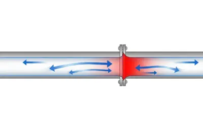
\begin{aligned} h_{f,1} (f_1) &= f_1 \frac{L_1}{D_1} h_{v1} \\ &= 0.0188 \times \frac{1600}{0.667} \times 0.18 \approx 8.10 \text{ ft} \end{aligned}

Calculate the contraction loss (based on downstream velocity $V_2$) :

\begin{aligned} h_{m,\text{contr.}} (K_c) &= K_c \cdot h_{v2} \\ &= 0.2 \times 0.56 \approx 0.11 \text{ ft} \end{aligned}

Calculate the friction loss for section 2:

\begin{aligned} h_{f,2} (f_2) &= f_2 \frac{L_2}{D_2} h_{v2} \\ &= 0.019 \times \frac{1000}{0.5} \times 0.56 \approx 21.14 \text{ ft} \end{aligned}

And finally, the exit loss (based on velocity $V_2$) :

\begin{aligned} h_{m,\text{exit}} (K_s) &= K_s \cdot h_{v2} \\ &= 1.0 \times 0.56 = 0.56 \text{ ft} \end{aligned}

Check: $ 0.09 + 8.10 + 0.11 + 21.14 + 0.56 = 30.00 \text{ ft} $. The sum of our calculated losses equals the total elevation drop. The calculation is consistent.

Building the Summary Table

We calculate the EGL and HGL at each point, starting from $EGL_A = 300 \text{ ft}$ and subtracting the losses. The velocity heads are $h_{v1} \approx 0.18 \text{ ft}$ and $h_{v2} \approx 0.56 \text{ ft}$.

Point A (Reservoir A Surface):

Total head is the surface elevation. Velocity is zero, so HGL = EGL.

\begin{aligned} EGL_A &= z_A = 300.00 \text{ ft} \\ HGL_A &= EGL_A - h_{vA} = 300.00 - 0 = 300.00 \text{ ft} \end{aligned}

Point 1 (After entrance):

EGL drops by the entrance loss ($h_{m,entry} \approx 0.09 \text{ ft}$). HGL is below EGL by the velocity head $h_{v1}$.

\begin{aligned} EGL_1 &= EGL_A - h_{m,entry} \\ &= 300.00 - 0.09 = 299.91 \text{ ft} \end{aligned}

\begin{aligned} HGL_1 &= EGL_1 - h_{v1} \\ &= 299.91 - 0.18 = 299.73 \text{ ft} \end{aligned}

Point 2 (Before contraction):

EGL drops by the friction loss in section 1 ($h_{f,1} \approx 8.10 \text{ ft}$). Velocity is still $V_1$.

\begin{aligned} EGL_2 &= EGL_1 - h_{f,1} \\ &= 299.91 - 8.10 = 291.81 \text{ ft} \end{aligned}

\begin{aligned} HGL_2 &= EGL_2 - h_{v1} \\ &= 291.81 - 0.18 = 291.63 \text{ ft} \end{aligned}

Point 3 (After contraction):

EGL drops by the contraction loss ($h_{m,contr.} \approx 0.11 \text{ ft}$). Velocity increases to $V_2$, so HGL drops further by $h_{v2}$.

\begin{aligned} EGL_3 &= EGL_2 - h_{m,contr.} \\ &= 291.81 - 0.11 = 291.70 \text{ ft} \end{aligned}

\begin{aligned} HGL_3 &= EGL_3 - h_{v2} \\ &= 291.70 - 0.56 = 291.14 \text{ ft} \end{aligned}

Point 4 (Before exit):

EGL drops by the friction loss in section 2 ($h_{f,2} \approx 21.14 \text{ ft}$). Velocity is still $V_2$.

\begin{aligned} EGL_4 &= EGL_3 - h_{f,2} \\ &= 291.70 - 21.14 = 270.56 \text{ ft} \end{aligned}

\begin{aligned} HGL_4 &= EGL_4 - h_{v2} \\ &= 270.56 - 0.56 = 270.00 \text{ ft} \end{aligned}

Point B (Reservoir B Surface):

EGL drops by the exit loss ($h_{m,exit} \approx 0.56 \text{ ft}$). The final EGL is 270.00 ft. Velocity becomes zero.

\begin{aligned} EGL_B &= EGL_4 - h_{m,exit} \\ &= 270.56 - 0.56 = 270.00 \text{ ft} \end{aligned}

\begin{aligned} HGL_B &= EGL_B - h_{vB} \\ &= 270.00 - 0 = 270.00 \text{ ft} \end{aligned}

We enter these values into the table:

Point	Description	Total Head (EGL) (ft)	Piezometric Head (HGL) (ft)
A	Reservoir A Surface	300.00	300.00
1	Just after entrance	299.91	299.73
2	Before contraction	291.81	291.63
3	Just after contraction	291.70	291.14
4	Just before exit	270.56	270.00
B	Reservoir B Surface	270.00	270.00

Schematic (After calculation)

EGL and HGL Plot

Reflections

The graph clearly shows the energy dissipation: the EGL (red line) continually drops. You can also see the effect of the contraction: velocity increases, so kinetic energy ($V^2/2g$) increases, and by conservation of energy, the pressure must drop, which makes the HGL (blue line) drop sharply.

Points of Caution

Make sure your EGL ends exactly at the elevation $z_B=270$ ft. If it doesn't, there is an error in the head loss calculation. Likewise, the HGL must meet the EGL at the reservoir surfaces, where velocity is zero.

Key Takeaways

The Energy Grade Line (EGL) can only go down (or stay level for a perfect fluid).
The Hydraulic Grade Line (HGL) can rise or fall depending on velocity changes.
The gap between the two lines is the kinetic energy (velocity head).

Did you know?

The "water hammer" phenomenon in pipes is directly related to these concepts. A sudden stop in flow (closing a valve) instantly converts all kinetic energy ($V^2/2g$) into a massive pressure surge, which can burst pipes. The HGL literally "hammers" upward.

FAQ

It's normal to have questions.

Final Result

The table and chart present the head values and the plots of the Energy Grade Line (EGL) and Hydraulic Grade Line (HGL) for the system.

Your Turn

Calculate the gage pressure (in psi) at point 2 (just before the contraction), assuming the pipe centerline elevation is 265 ft. (Hint: $P_{\text{psi}} = (HGL - z_{\text{pipe}}) / 2.31$).

Interactive Tool: Influence of Diameter

Use the simulator to observe how the diameter of the second section ($D_2$) and the total elevation drop ($\Delta z = z_A - z_B$) influence the flow rate and head loss. A smaller diameter or a smaller elevation drop increases resistance and reduces the flow rate.

Input Parameters

Elevation Drop $ \Delta z $ (ft) 30 ft

Diameter $ D_2 $ (in) 6.0 in

Key Results

Discharge $Q_v$ (cfs) -

Velocity $V_1$ (ft/s) -

Energy Grade Line (EGL): A line representing the total head (or total energy per unit weight) of the fluid at each point in the flow. Its elevation is given by $ H_t = z + P/\gamma + V^2/(2g) $.
Hydraulic Grade Line (HGL): A line representing the piezometric head (the sum of elevation and pressure head) at each point. Its elevation is given by $ H_p = z + P/\gamma $. It corresponds to the level water would rise to in a piezometer tube attached to the pipe.
Head Loss: The irreversible loss of energy (converted to heat) experienced by the fluid, primarily due to friction (major/friction losses) and pipe components (minor losses).

Total Head Loss in a Simple Pipe System

Fundamentals of Hydraulics

Exercise: Total Head Loss in a Simple Pipe System Calculating Total Head Loss in a Simple Pipe System Context: Water Flow in Pipes. In hydraulics, particularly in civil engineering fields like potable water supply or sanitation systems, it is crucial to understand and...

Calculating Singular Head Loss for a Valve

Fundamentals of Hydraulics

Exercise: Singular Head Loss for a Valve Calculating Singular Head Loss for a Valve Context: Singular Head LossLocalized energy losses in a hydraulic circuit, caused by pipe fittings (elbows, valves, tees, etc.) that disrupt the fluid flow.. In any hydraulic circuit,...

Comparison of Hydraulic Head Loss

Fundamentals of Hydraulics

Exercise: Comparing Hydraulic Head Loss Comparison of Hydraulic Head Loss Context: Fundamentals of Pressurized Pipe Flow. Transporting fluids in pipes is a pillar of civil and industrial engineering. However, as a fluid flows, it inevitably loses energy due to...

Calculating Power Dissipated by Head Loss

Fundamentals of Hydraulics

Exercise: Power Dissipated by Head Loss Calculating the Power Dissipated by Head Loss Context: Energy in Fluid Flow. When a fluid flows through a pipe, it loses energy due to friction against the walls (major head loss) and obstacles such as elbows, valves, or...

Head Loss Calculation with Hazen-Williams

Fundamentals of Hydraulics

Exercise: Head Loss Calculation with Hazen-Williams Head Loss Calculation with Hazen-Williams Context: Sizing a Water Supply Pipeline. One of the major challenges in hydraulic engineering is transporting water over long distances efficiently. To do this, it's crucial...

Influence of Viscosity on Head Loss

Fundamentals of Hydraulics

Influence of Viscosity on Head Loss (US Customary Units) Influence of Viscosity on Head Loss Context: Fluid Flow in Pipes. Transporting fluids (water, oil, gas, etc.) through pipelines is ubiquitous in industry and daily life. During this flow, the fluid rubs against...

Falling Sphere Velocity according to Stokes’ Law

Fundamentals of Hydraulics

Exercise: Falling Sphere Velocity (Stokes' Law) Falling Sphere Velocity according to Stokes' Law Context: Studying Stokes' LawFormula expressing the drag force on a sphere moving in a viscous fluid at low velocity.. In fluid mechanics, understanding the motion of an...

Calculating a Pump’s Maximum Suction Head

Fundamentals of Hydraulics

Calculating Maximum Suction Head Calculating a Pump's Maximum Suction Head Context: One of the biggest challenges in hydraulics is ensuring a pump operates correctly by avoiding the destructive phenomenon of cavitationThe formation of vapor bubbles in a liquid when...

Analysis of Temperature Effects in Hydraulics

Fundamentals of Hydraulics

Exercise: Impact of Temperature on Head Loss Analysis of Temperature Effects in Hydraulics Context: The Impact of Thermal Variations on Hydraulic Systems. In many industrial applications, from petrochemicals to HVAC, fluids are transported at widely varying...

← Interpreting a Log Splitter Hydraulic Schematic Volumetric Efficiency of a Worn Pump →