Calculating Total Head Loss in a Simple Pipe System
Context: Water Flow in Pipes.
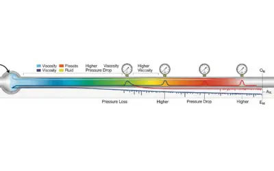
In hydraulics, particularly in civil engineering fields like potable water supply or sanitation systems, it is crucial to understand and quantify the energy lost by a fluid as it flows through a pipe. This energy loss, known as head lossThe reduction in the total head (sum of elevation, pressure, and velocity head) of a fluid as it moves through a pipe system due to friction (major losses) and components like bends and valves (minor losses)., is caused by the friction of the fluid against the pipe walls (major or friction losses) and by obstacles that disrupt the flow, such as bends, valves, or changes in cross-section (minor or singular losses). A precise calculation of these losses is essential for correctly sizing pumps or ensuring that gravity flow is feasible.
Pedagogical Note: This exercise will guide you through the fundamental steps of calculating the total head loss in a simple piping system, applying principles of fluid mechanics and standard industry formulas.
Learning Objectives
- Understand the difference between major (friction) and minor (singular) head losses.
- Apply the Darcy-Weisbach equation to calculate friction losses.
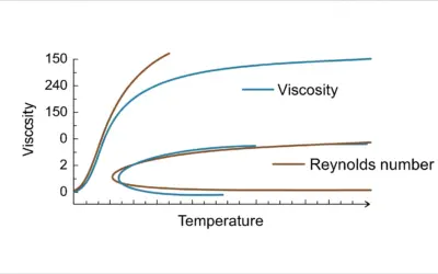
- Calculate the Reynolds numberA dimensionless quantity used to predict flow patterns. It characterizes the flow as laminar or turbulent. to determine the flow regime.
- Determine the friction factorA dimensionless coefficient used in the Darcy-Weisbach equation, which depends on the pipe's roughness and the Reynolds number. using an approximation of the Colebrook-White equation.
- Calculate the total energy dissipated in a simple pipe.
Problem Data
Installation Diagram
| Characteristic | Symbol | Value |
|---|---|---|
| Volumetric Flow Rate | \(Q\) | 317 GPM (Gallons Per Minute) |
| Inner Pipe Diameter | \(D\) | 4.0 in |
| Total Pipe Length | \(L\) | 500 ft |
| Pipe Material | - | Cast Iron |
| Absolute Roughness (Cast Iron) | \(\epsilon\) | 0.000853 ft |
| Kinematic Viscosity (Water @ 50°F) | \(\nu\) | \(1.41 \times 10^{-5}\) ft²/s |
| Acceleration of Gravity | \(g\) | 32.2 ft/s² |
| Fittings on the line | \(\sum K\) | 2 std. 90° elbows (\(K=0.9\)) and 1 open gate valve (\(K=0.2\)) |
Problem Questions
- Calculate the flow velocity (\(V\)) and the Reynolds number (\(Re\)).
- Determine the friction factor (\(f\)) using an approximation of the Colebrook-White equation.
- Calculate the major (friction) head losses (\(h_f\)).
- Calculate the sum of the minor (singular) head losses (\(h_s\)).
- Determine the total head loss (\(H_T\)) of the system.
Fundamentals of Head Loss
The total head loss (\(H_T\)) in a pipe is the sum of major (friction) losses (\(h_f\)) and minor (singular) losses (\(h_s\)).
1. Flow Regime and Reynolds Number (\(Re\))
The Reynolds number is a dimensionless quantity that helps determine if a flow is laminar (low velocities, smooth streamlines) or turbulent (high velocities, chaotic eddies).
\[ Re = \frac{V \cdot D}{\nu} \]
Where \(V\) is velocity (ft/s), \(D\) is diameter (ft), and \(\nu\) is kinematic viscosity (ft²/s). If \(Re < 2000\), the flow is laminar. If \(Re > 4000\), it is turbulent.
2. Major (Friction) Losses (\(h_f\)) and the Darcy-Weisbach Equation
These are due to the friction of the fluid along the entire length of the pipe. They are calculated using the Darcy-Weisbach equation:
\[ h_f = f \cdot \frac{L}{D} \cdot \frac{V^2}{2g} \]
Where \(f\) is the friction factor, \(L\) is the length (ft), \(D\) is the diameter (ft), \(V\) is the velocity (ft/s), and \(g\) is the acceleration of gravity (ft/s²).
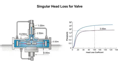
3. Minor (Singular) Losses (\(h_s\))
These are localized at pipe fittings (bends, valves, etc.). Each fitting is characterized by a loss coefficient K.
\[ h_s = \sum K \cdot \frac{V^2}{2g} \]
Where \(\sum K\) is the sum of the coefficients for all fittings in the line.
Solution: Total Head Loss in a Simple Pipe System
Question 1: Calculate velocity (\(V\)) and Reynolds number (\(Re\))
Principle
The first step is to determine the basic characteristics of the flow. Velocity is directly related to the flow rate and the pipe's cross-sectional area (principle of conservation of mass). The Reynolds number will then tell us if the flow is smooth (laminar) or chaotic (turbulent), which is crucial for all subsequent calculations.
Mini-Course
The continuity equation for an incompressible fluid (\(Q = V \times A\)) states that the flow rate is constant. The Reynolds number physically compares inertial forces (which tend to create chaos and turbulence) to viscous forces (which tend to dampen motion and keep it orderly and laminar). A high Re means inertia dominates, hence turbulence.
Pedagogical Note
Always start with these preliminary calculations. They lay the foundation for the entire analysis. An error here will propagate to all following results. Correctly determining the flow regime (laminar or turbulent) is the most critical step.
Standards
While there isn't a regulatory standard for this basic calculation, the values for fluid properties (like the viscosity of water at a given temperature) are standardized in international reference tables (e.g., IAPWS - International Association for the Properties of Water and Steam).
Formulas
Velocity Formula
Reynolds Number Formula
Assumptions
For these calculations, we make the following assumptions:
- The fluid (water) is incompressible.
- The flow is steady (flow rate does not change over time).
- The velocity is uniform across the pipe's cross-section (an approximation for average velocity).
Given Data
We extract the necessary data from the problem statement:
| Parameter | Symbol | Value | Unit |
|---|---|---|---|
| Volumetric Flow Rate | \(Q\) | 317 | GPM |
| Inner Diameter | \(D\) | 4.0 | in |
| Kinematic Viscosity | \(\nu\) | \(1.41 \times 10^{-5}\) | ft²/s |
Tips
In typical water supply systems, velocities are generally between 2 and 8 ft/s. If your velocity calculation falls far outside this range, double-check your units!
Diagram (Before Calculations)
Velocity Visualization in the Pipe
Calculations
1. Unit Conversions
We must first convert the flow rate and diameter to standard USCS units (ft³/s and ft). First, the flow rate (1 ft³ ≈ 7.48 gal, 1 min = 60 s):
Next, convert the diameter (1 ft = 12 in):
2. Calculate Cross-Sectional Area (\(A\))
Using the formula for the area of a circle \(A = \pi D^2 / 4\) with the diameter in feet:
The cross-sectional area of the pipe is approximately 0.0872 ft².
3. Calculate Velocity (\(V\))
Using the relationship \(Q = V \times A\), so \(V = Q / A\). We use the values in ft³/s and ft²:
The average water velocity in the pipe is 8.10 ft/s.
4. Calculate Reynolds Number (\(Re\))
Apply the formula \(Re = VD/\nu\) using the calculated velocity, diameter in feet, and kinematic viscosity:
The number is dimensionless. Since \(191,200 > 4000\), the flow is turbulent.
Diagram (After Calculations)
Turbulent Flow Visualization
Reflections
The Reynolds number is 191,200. As this value is much greater than 4000, we can conclude that the flow is in the turbulent regime. This information is essential because the calculation of the friction factor depends on it.
Points of Vigilance
The most common error here is unit conversion. Ensuring the flow rate is in ft³/s (cfs) and the diameter is in ft before any calculation is imperative to avoid an incorrect result by several orders of magnitude.
Key Takeaways
- Velocity is derived from flow rate using \(V=Q/A\).
- The Reynolds number (\(Re = VD/\nu\)) is the criterion that defines the flow regime.
- \(Re > 4000 \Rightarrow\) Turbulent Flow.
Did you know?
The experiment that visualized the transition between laminar and turbulent flow was conducted by British engineer Osborne Reynolds in 1883. He injected a dye filament into a clear glass tube to observe the fluid's behavior at different velocities.
FAQ
Final Result
Try it yourself
If the flow rate were reduced to 100 GPM, what would be the new velocity?
Question 2: Determine the friction factor (\(f\))
Principle
The friction factor \(f\) quantifies the flow resistance due to the pipe wall's roughness. In the turbulent regime, it depends on both the Reynolds number (the intensity of turbulence) and the pipe's relative roughness (\(\epsilon/D\), the significance of the wall's microscopic "bumps" compared to the pipe's diameter).
Mini-Course
The most accurate relationship for the friction factor in turbulent flow is the Colebrook-White equation. It is an "implicit" equation: the term \(f\) we are looking for appears on both sides, meaning we cannot isolate it directly. To solve it, we must use an iterative numerical method: we start with an estimate, plug it into the formula to get a new one, and repeat the process until the value stabilizes (converges).
Pedagogical Note
The choice of the correct formula is dictated by the flow regime. For laminar flow, the formula would be much simpler (\(f=64/Re\)). Since we are in the turbulent regime, a more complex formula is necessary. The iterative method, though longer, is the standard for obtaining an accurate result.
Standards
The absolute roughness values (\(\epsilon\)) for various pipe materials (cast iron, PVC, steel...) are tabulated in engineering standards and fluid mechanics textbooks. It's important to choose the value corresponding to the material and condition of the pipe (new or aged).
Formulas
Colebrook-White Equation (Implicit)
Haaland Equation (for initial guess)
Assumptions
We assume the given roughness value of \(\epsilon = 0.000853\) ft is uniform and representative of the pipe's condition along its entire length.
Given Data
We use the results from the previous question and the problem statement:
| Parameter | Symbol | Value | Unit |
|---|---|---|---|
| Reynolds Number | \(Re\) | 191,200 | - |
| Absolute Roughness | \(\epsilon\) | 0.000853 | ft |
| Inner Diameter | \(D\) | 0.333 | ft |
Tips
A good initial guess allows for faster convergence to the solution. The Haaland equation is an excellent candidate for this. Usually, 2 or 3 iterations are sufficient for excellent accuracy.
Diagram (Before Calculations)
Relative Roughness Concept
Calculations
1. Calculate Relative Roughness (\(\epsilon/D\))
This is the ratio of the roughness height to the pipe diameter. Both must be in the same unit (feet). This ratio is dimensionless.
2. Solve Colebrook-White via Iteration
The equation \(\frac{1}{\sqrt{f}} = -2 \log_{10}\left(\frac{\epsilon/D}{3.7} + \frac{2.51}{Re\sqrt{f}}\right)\) cannot be solved directly. We use a starting guess and refine the result with each step.
Step 2a: Initial Guess (\(f_0\)) with Haaland
We use the Haaland equation to find a reasonable starting \(f_0\). We plug in \(\epsilon/D = 0.00256\) and \(Re = 191,200\):
Now, we solve for \(f_0\) by taking the inverse square:
Our first guess is \(f_0 \approx 0.0232\).
Step 2b: Iteration 1 (Calculate \(f_1\))
We plug \(f_0 = 0.0232\) into the right side of the Colebrook-White equation to find a better approximation, \(f_1\):
Solve for \(f_1\):
This new value \(f_1 = 0.0258\) is different from \(f_0\). We continue iterating.
Step 2c: Iteration 2 (Calculate \(f_2\))
We repeat the process, plugging the new value \(f_1 = 0.0258\) into the right side:
Solve for \(f_2\):
The value \(f_2 = 0.0257\) is very close to \(f_1 = 0.0258\). We can stop here. The value has converged.
Step 2d: Final Value
We will use \(f \approx 0.0257\).
Diagram (After Calculations)
Position on the Moody Diagram
Reflections
The value converged quickly to \(f \approx 0.0257\). This value is directly related to the amount of energy that will be lost to friction over the length of the pipe. A smoother pipe (like PVC) would have a lower \(\epsilon/D\) and thus a lower friction factor.
Points of Vigilance
Be careful with relative roughness: \(\epsilon\) and \(D\) must be in the same unit (in this case, feet) before calculating the ratio. Forgetting this step is a common source of error.
Key Takeaways
- In turbulent flow, \(f\) depends on both \(Re\) and \(\epsilon/D\).
- The Colebrook-White equation is the most accurate but requires an iterative solution.
Did you know?
The Moody Diagram, which graphically represents the friction factor, was created in 1944 by Lewis Ferry Moody. It remains a fundamental tool for hydraulic engineers worldwide, even in the age of numerical computation.
FAQ
Final Result
Try it yourself
If the pipe were smooth PVC (\(\epsilon = 0.000005\) ft), what would the approximate new friction factor \(f\) be?
Question 3: Calculate the major (friction) head losses (\(h_f\))
Principle
Major (or friction) losses represent the energy dissipated by friction over the entire length of the pipe. It's like a continuous braking force acting on the fluid. We will quantify this "energy head loss" using the Darcy-Weisbach equation, which relates this loss to the friction factor, the pipe dimensions, and the fluid's kinetic energy.
Mini-Course
The term \(V^2/(2g)\) is called the "velocity head". It represents the kinetic energy of the fluid per unit weight. The Darcy-Weisbach equation shows that friction loss is proportional to this kinetic energy, the length of the pipe, and inversely proportional to its diameter.
Pedagogical Note
In long-distance pipelines, such as in water supply or civil engineering networks, friction losses almost always constitute the largest portion of the total losses. Their accurate calculation is therefore paramount.
Standards
The Darcy-Weisbach equation is universally accepted and forms the basis of all hydraulic piping calculation codes and standards worldwide, including in the U.S.
Formulas
Darcy-Weisbach Equation
Assumptions
We assume that the friction factor \(f\) we calculated is constant over the entire length \(L\) of the pipe.
Given Data
We gather all the necessary values:
| Parameter | Symbol | Value | Unit |
|---|---|---|---|
| Friction Factor | \(f\) | 0.0257 | - |
| Length | \(L\) | 500 | ft |
| Diameter | \(D\) | 0.333 | ft |
| Velocity | \(V\) | 8.096 | ft/s |
| Gravity | \(g\) | 32.2 | ft/s² |
Tips
Calculate the velocity head term \(V^2/(2g)\) first, as it will be reused for calculating minor losses. This avoids redundant calculations.
Diagram (Before Calculations)
Visualization of Friction Forces
Calculations
1. Calculate Velocity Head
This term \(V^2 / 2g\) represents the kinetic energy of the fluid (per unit weight). We calculate it first as it will be reused:
2. Calculate Major (Friction) Head Loss (\(h_f\))
We apply the Darcy-Weisbach formula by plugging in the friction factor \(f\), the ratio \(L/D\), and the velocity head:
Substituting the numerical values:
The energy loss due to friction over the 500 ft of pipe is 39.24 feet of head.
Diagram (After Calculations)
Drop in the Energy Grade Line (Friction)
Reflections
A loss of 39.24 feet means that the energy in the water has dropped by an amount equivalent to falling 39.24 ft, just to overcome friction. This is a significant energy loss that must be supplied by a pump or an elevation difference (gravity).
Points of Vigilance
Ensure all units are in the standard USCS system (feet, seconds) before applying the formula. A conversion error on length \(L\) or diameter \(D\) is common.
Key Takeaways
- Friction losses are calculated using the Darcy-Weisbach equation.
- They are proportional to the length \(L\) and the friction factor \(f\).
- They are inversely proportional to the diameter \(D\).
Did you know?
French engineer Henry Darcy conducted his experiments on water flow through sand beds in Dijon in 1856, laying the groundwork for modern hydrodynamics and hydrology. The equation was later refined by Saxon engineer Julius Weisbach.
FAQ
Final Result
Try it yourself
If the pipe were only 100 ft long, what would the friction head loss \(h_f\) be?
Question 4: Calculate the minor (singular) head losses (\(h_s\))
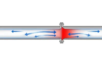
Principle
Minor losses represent the energy lost due to local disturbances in the flow. Each fitting (bend, valve, etc.) forces the fluid to change direction or velocity, which generates intense turbulence that dissipates energy as heat. We sum the effects of each fitting to get the total minor loss.
Mini-Course
The loss coefficient \(K\) is a dimensionless number determined experimentally. It represents the multiple of the velocity head (\(V^2/2g\)) that is lost as the fluid passes through the fitting. The higher the \(K\), the more obstructive the fitting is to the flow.
Pedagogical Note
Although often smaller than friction losses in long pipelines, minor losses can become dominant in short, complex systems with many fittings, such as in pump houses or mechanical rooms.
Standards
Loss coefficients \(K\) for thousands of standard fittings (bends, tees, valves, reducers...) are listed in engineering handbooks like the "Crane Technical Paper No. 410" or ISO standards.
Formulas
Minor Loss Formula
Assumptions
We assume the handbook K-values are applicable to our case. We also neglect interactions between fittings (i.e., we assume they are spaced far enough apart for the flow to stabilize between them).
Given Data
Data is from the problem statement and previous calculations:
- Std. 90° elbow: \(K = 0.9\) (x2)
- Open gate valve: \(K = 0.2\)
- Velocity head: \(V^2/(2g) \approx 1.018\) ft
Tips
To simplify, group all identical fittings. Here, we have 2 elbows, so their contribution is \(2 \times K_{\text{elbow}}\). The sum of all \(K\) values is a good indicator of a circuit's hydraulic "complexity".
Diagram (Before Calculations)
Examples of Turbulence-Inducing Fittings
Calculations
1. Sum of K-Coefficients
We add the loss coefficients for all listed fittings (2 elbows and 1 valve):
The sum of the minor loss coefficients is 2.0.
2. Calculate Minor Head Loss (\(h_s\))
We apply the formula \(h_s = (\sum K) \cdot (V^2 / 2g)\) using the velocity head \(V^2 / 2g\) calculated in Question 3 (which was 1.018 ft):
Substituting the values:
The energy loss due to fittings is 2.04 feet of head.
Diagram (After Calculations)
Drops in the Energy Grade Line (Major + Minor)
Reflections
The loss due to fittings is 2.04 ft. Compared to the friction loss of 39.24 ft, it is small (about 5% of the friction loss). This confirms that for this long pipe, friction along the length is the dominant factor in energy loss.
Points of Vigilance
A common mistake is forgetting a fitting or using the wrong K-coefficient. These coefficients are empirical and must be chosen carefully from reference tables based on the exact type of fitting (e.g., a long-radius elbow has a much lower K-value than a standard elbow).
Key Takeaways
- Minor losses are localized at pipe "events" or fittings.
- Each fitting is characterized by a \(K\) coefficient.
- The total minor loss is \(\sum K \times V^2/(2g)\).
Did you know?
Modern hydraulic design, aided by Computational Fluid Dynamics (CFD), can accurately simulate flow through complex geometries and calculate head losses with high precision, reducing the reliance on simple tabulated K-coefficients.
FAQ
Final Result
Try it yourself
If a check valve (\(K=2.5\)) were added to the line, what would the new minor loss \(h_s\) be?
Question 5: Determine the total head loss (\(H_T\))
Principle
The total head loss is simply the arithmetic sum of the two types of losses we just calculated: the continuous losses from friction (major) and the localized losses from fittings (minor). This represents the total energy dissipation of the system.
Mini-Course
In the general energy equation (an extension of Bernoulli's equation), \(H_T\) represents the energy loss term. For flow to occur, the sum of the pressure head, velocity head, and elevation head at the starting point must be greater than the sum of those same heads at the end point, plus the total head loss between them. \(H_T\) is the energy that was "lost" (converted to heat).
Pedagogical Note
This final value is what's crucial for the engineer. It is used to determine the total dynamic head (TDH) a pump must provide, or to verify if an elevation difference (gravity) is sufficient to maintain the required flow rate.
Standards
Design standards for water supply networks (like AWWA standards) impose rules on maximum velocities to limit head loss and the risk of water hammer, thereby indirectly influencing the maximum acceptable value for \(H_T\).
Formulas
Total Head Loss Formula
Assumptions
We assume there are no other un-accounted-for sources of loss in our analysis.
Given Data
We use the final results from Questions 3 and 4.
| Parameter | Symbol | Value | Unit |
|---|---|---|---|
| Major (Friction) Loss | \(h_f\) | 39.24 | ft |
| Minor (Singular) Loss | \(h_s\) | 2.04 | ft |
Diagram (Before Calculations)
Summing the Major and Minor Losses
Calculations
Calculate Total Head Loss (\(H_T\))
This is the simple sum of the major losses (from friction over the length) and the minor losses (from fittings):
We add the results from Questions 3 and 4:
The total head loss for the entire system is 41.28 ft.
Diagram (After Calculations)
Resulting Total Energy Grade Line
Reflections
The total head loss is 41.28 ft. This means that a "push" equivalent to a 41.28-foot column of water (or about 17.9 psi) is required just to overcome the flow resistance and maintain the 317 GPM flow rate. This energy must be supplied either by a pump or by an elevation difference between the start and end points.
Points of Vigilance
The error here would be to neglect one of the two types of losses. Even though the minor losses are small in this case, they can be significant in other configurations and should never be forgotten.
Key Takeaways
- Total head loss is the sum of major (friction) and minor (singular) losses.
- \(H_T = h_f + h_s\).
- This value represents the total energy that must be supplied to the system to maintain the flow.
Did you know?
Optimizing a network to reduce head loss is a major economic and environmental goal. A small reduction in losses on a large water distribution network operating 24/7 can represent thousands of dollars in annual energy savings and reduce the city's carbon footprint.
FAQ
Final Result
Try it yourself
Using the results from the previous 'Try it yourself' sections (100 ft pipe and added check valve), what would the new total head loss (H_T) be?
Interactive Tool: Head Loss Simulator
Use the sliders to vary the flow rate and pipe length, and observe their impact on the major and total head losses. The diameter (4.0 in) and roughness (0.000853 ft) remain fixed.
Input Parameters
Key Results
Final Quiz: Test Your Knowledge
1. What primary parameter is used to distinguish laminar from turbulent flow?
2. "Minor" or "singular" head losses are primarily caused by:
3. If you double the length of a pipe (all other parameters remaining identical), how will the major (friction) head losses change?
4. In the turbulent flow regime, what does the friction factor \(f\) depend on?
5. Increasing the pipe diameter, for the same flow rate, will tend to:
Glossary
- Head Loss
- The loss of energy (expressed as a height of fluid, e.g., feet of head) experienced by a fluid as it flows through a pipe system, due to friction and fittings.
- Reynolds Number (Re)
- A dimensionless quantity that characterizes the flow regime (laminar, transitional, turbulent). It represents the ratio of inertial forces to viscous forces.
- Roughness (\(\epsilon\))
- A measure of the surface imperfections on a pipe's interior wall, which influences fluid friction. It is typically given in feet or millimeters.
- Friction Factor (f)
- A dimensionless coefficient used in the Darcy-Weisbach equation to calculate friction losses. It is also known as the major loss coefficient.


0 Comments